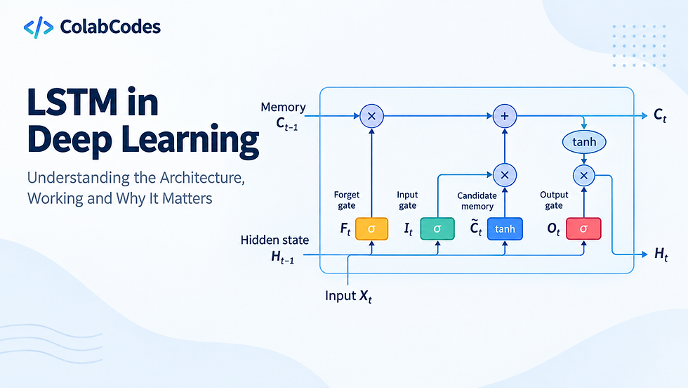
GRU in Deep Learning: Architecture, Working, and Implementation in Python

Gated Recurrent Units (GRUs) are a type of recurrent neural network architecture designed to model sequential data while addressing some of the optimization difficulties associated with conventional RNNs. Introduced by Cho et al. in 2014 as part of the RNN Encoder-Decoder framework, GRUs use gating mechanisms to control how information from previous time steps is retained, updated, and incorporated into the current hidden state.

GRUs belong to the same family of gated recurrent architectures as Long Short-Term Memory (LSTM) networks. Their central idea is to regulate the flow of information through the hidden state rather than replacing the recurrent mechanism entirely. Compared with LSTMs, GRUs use a simpler state representation and fewer gates, resulting in a more compact recurrent architecture. Empirical work by Chung et al. found GRUs to be competitive with LSTMs on sequence-modeling tasks.

This article examines the motivation behind GRUs, their architecture, the update and reset gates, the mathematical formulation of a GRU cell, its step-by-step operation, its differences from RNNs and LSTMs, and its implementation in Python using PyTorch.

What Is a GRU in Deep Learning?

A Gated Recurrent Unit is a gated recurrent neural network that computes a hidden state at each time step using the current input and the hidden state from the previous time step. The gating mechanism determines how much of the previous hidden representation should be retained and how much new information should be incorporated.

A conventional RNN updates its hidden state using a recurrent transformation such as:

hₜ = tanh ( Wx xₜ + Wₕ hₜ₋₁ + b )

where xₜ is the input at time t,  hₜ₋₁ is the previous hidden state, and hₜ is the current hidden state.

Although this formulation allows information to propagate through a sequence, repeated nonlinear transformations can make optimization difficult over long sequences. In particular, gradients can become extremely small or excessively large during backpropagation through time, making it difficult for a basic RNN to learn long-range dependencies.

GRUs introduce gates that allow the network to learn how information should flow through the recurrent computation. Instead of forcing every previous hidden representation to be completely transformed at every step, the network can preserve useful information and selectively replace outdated information.

Why Were GRUs Introduced?

The motivation behind GRUs is closely related to the same problem that motivated gated architectures such as LSTMs: conventional recurrent networks can struggle with dependencies that span many time steps.

For a long sequence, information from an early position has to pass through many recurrent operations before influencing a later prediction. During training, gradients associated with these long computational paths can progressively diminish, contributing to the vanishing-gradient problem.

LSTMs address this through a separate cell state and several gates. GRUs take a more compact approach. Instead of maintaining a separate cell state, a GRU stores its recurrent information in a single hidden state and uses two principal gates:

• the update gate

• the reset gate

These gates allow a GRU to preserve historical information, replace it with new information, or temporarily reduce the influence of previous information.

GRU Architecture

At every step in a temporal sequence, a Gated Recurrent Unit (GRU) functions as an information filter. It continuously ingests two primary inputs: the current external feature vector xₜ and the compressed context vector from the immediate past, known as the previous hidden state hₜ₋₁. From these inputs, it computes an updated hidden state hₜ, which serves both as the output representation for step t and as the temporal memory passed forward to step t+1. he standard mathematical formulation used in production frameworks such as PyTorch defines the precise sequence of operations as follows:

rₜ = σ ( Wir xt + bir + Whr hₜ₋₁ + bhr )

zₜ = σ ( Wiz xt + biz + Whz hₜ₋₁ + bhz )

nₜ = tanh ( Win xt + bin + rt ⊙ Whn hₜ₋₁ + bhn )

hₜ = ( 1 - zₜ ) ⊙ nₜ + zₜ ⊙ hₜ₋₁

Here, σ denotes the sigmoid function and ⊙ denotes element-wise multiplication.

The exact arrangement of the reset operation can differ between the original GRU formulation and framework implementations. PyTorch explicitly notes that its implementation applies the reset gate after the hidden-to-hidden matrix multiplication for computational efficiency, whereas the original formulation applies the reset operation to the previous hidden state before that multiplication.

The Reset Gate

The reset gate determines how strongly the previous hidden state contributes to the generation of new information. It is calculated as:

rₜ = σ ( Wir xt + bir + Whr hₜ₋₁ + bhr )

Because the sigmoid function produces values between 0 and 1, the reset gate can be interpreted as a learned element-wise filter. A value close to 1 allows more information from the previous hidden state to participate in the candidate computation. A value close to 0 reduces the influence of that previous information. The reset gate therefore provides the network with a mechanism for selectively disregarding parts of the previous representation when constructing the new candidate state.

Conceptually, this is useful when the information relevant to the current input is different from information represented in the recent history. The network does not have to completely discard the previous hidden state; it can control its contribution dimension by dimension.

The Update Gate

The update gate determines how the previous hidden state and the newly computed candidate state are combined. It is calculated as:

zₜ = σ ( Wiz xt + biz + Whz hₜ₋₁ + bhz )

The final hidden state is then:

hₜ = ( 1 - zₜ ) ⊙ nₜ + zₜ ⊙ hₜ₋₁

This equation is one of the defining characteristics of a GRU.

When an element of zₜ approaches 1, more of the previous hidden state is retained. When it approaches 0, more of the candidate state is incorporated. The update gate therefore controls the degree of change applied to the recurrent representation.

It is useful to think of the update gate as a learned mechanism for deciding how much historical information remains relevant at the current step. This allows the network to preserve useful information across many recurrent transitions instead of continuously overwriting it.

Candidate Hidden State

After calculating the reset and update gates, the GRU constructs a candidate hidden representation:

nₜ = tanh ( Win xt + bin + rt ⊙ Whn hₜ₋₁ + bhn )

The reset gate appears directly in this calculation. The candidate state represents the new information that could be incorporated into the recurrent representation. It depends on both the current input and a gated version of the previous hidden state.

The hyperbolic tangent function maps the resulting activation into the range [-1,1], producing a bounded candidate representation. The GRU then combines this candidate with the previous hidden state through the update gate.

Putting it all together

At time step t, the GRU follows a repeated sequence of operations. First, the current input xt and the previous hidden state hₜ₋₁ are provided to the recurrent unit. The network computes the reset gate rt. This determines how strongly the previous state participates in the creation of new information.

Next, the update gate zₜ is calculated. This determines the relative contribution of the previous hidden state and the candidate state. The candidate state nₜ is then generated using the current input and the reset-controlled previous representation.

Finally, the previous hidden state and candidate state are interpolated to produce the new hidden state ht. This process is repeated for every element of the sequence.

The important characteristic is that the GRU does not have to completely replace hₜ₋₁ at every time step. Through the update gate, information can persist across many steps.

GRU vs RNN vs LSTM

GRUs are best understood in relation to the recurrent architectures that preceded them.

A standard RNN typically has a relatively simple recurrent update and no explicit gating mechanism. LSTM introduces multiple gates and a dedicated cell state, while GRU combines recurrent memory and gating into a simpler structure.

Characteristic	RNN	GRU	LSTM
Gating	No	Update + reset	Input + forget + output
Separate cell state	No	No	Yes
Hidden state	Yes	Yes	Yes
Number of main recurrent states	1	1	2
Architecture complexity	Low	Moderate	Higher
Long-term dependency handling	Limited	Stronger	Stronger
Parameter count	Lowest	Generally lower than LSTM	Generally higher
Typical computation	Simple	Efficient gated computation	More extensive gated computation

The empirical study by Chung et al. compared GRUs and LSTMs with traditional recurrent units and reported that gated recurrent units performed better than traditional tanh-based recurrent units in the investigated sequence-modeling experiments, while GRUs were comparable to LSTMs.

The lower architectural complexity of a GRU does not imply that it is universally superior to an LSTM. The appropriate recurrent architecture depends on the sequence characteristics, dataset, computational constraints, and task.

GRU Parameterization

One practical advantage of the GRU architecture is its relatively compact parameterization.

For each recurrent layer, the GRU maintains learned weights for the reset gate, update gate, and candidate state.

Because the GRU does not maintain a separate cell state and uses fewer gates than an LSTM, it generally requires fewer parameters for equivalent input and hidden dimensions. This can make GRUs attractive when computational efficiency and model size are important considerations.

Implementing a GRU in Python with PyTorch

PyTorch provides GRU functionality through torch.nn.GRU. The layer accepts the input feature size and hidden-state size as its primary architectural parameters. It can also be configured using arguments such as num_layers, dropout, batch_first, and bidirectional.

A basic GRU model for sequence classification can be implemented as follows:

import torch
import torch.nn as nn


class GRUClassifier(nn.Module):
    def __init__(self, input_size, hidden_size, num_classes):
        super().__init__()

        self.gru = nn.GRU(
            input_size=input_size,
            hidden_size=hidden_size,
            batch_first=True
        )

        self.fc = nn.Linear(hidden_size, num_classes)

    def forward(self, x):
        output, hidden = self.gru(x)
        final_hidden = hidden[-1]

        return self.fc(final_hidden)

Suppose each sequence contains 20 time steps and every time step has 10 features. A model can be created with:

model = GRUClassifier(
    input_size=10,
    hidden_size=64,
    num_classes=3
)

With batch_first=True, the input is expected in the shape:

(batch_size, sequence_length, input_size)

For example:

x = torch.randn(32, 20, 10)

output = model(x)

print(output.shape)

The resulting output has the shape:

(32, 3)

Here, 32 represents the batch size and 3 represents the number of output classes.

PyTorch returns both the sequence of hidden representations and the final hidden state from nn.GRU. The output tensor contains the hidden representation from the last GRU layer for every time step, while h_n contains the final hidden state for each recurrent layer and direction.

Stacked and Bidirectional GRUs

A GRU does not have to consist of a single recurrent layer.

Multiple GRU layers can be stacked:

gru = nn.GRU(
    input_size=10,
    hidden_size=64,
    num_layers=2,
    batch_first=True
)

The first GRU layer processes the original sequence, while the second layer processes the hidden representations produced by the first layer.

GRUs can also be bidirectional:

gru = nn.GRU(
    input_size=10,
    hidden_size=64,
    batch_first=True,
    bidirectional=True
)

A bidirectional GRU processes the sequence in both forward and reverse directions. Consequently, its output feature dimension becomes twice the hidden size because representations from both directions are combined.

This can be useful for tasks where information from both earlier and later positions in a sequence is available during prediction.

GRUs and the Evolution of Sequence Models

While Gated Recurrent Units streamline sequence modeling, their core architecture imposes distinct trade-offs when evaluated against alternative neural network designs:

1. Sequential Bottleneck: Because GRUs are inherently recurrent, computing state ht strictly requires state ht-1. This step-by-step dependency prevents parallel processing across sequence positions during training, creating a major computational throughput bottleneck on modern GPU hardware.

2. Simplified Capacity: The unified hidden state makes GRUs computationally lightweight, but it can limit model capacity for complex, long-range dependencies compared to LSTMs, which maintain an isolated cell state alongside three distinct control gates.

3. Task-Dependent Performance: In practice, neither architecture strictly outperforms the other; empirical results depend heavily on dataset scale, temporal density, and domain constraints.

   
   

For large-scale sequence tasks, modern deep learning has largely shifted toward Transformer architectures. By leveraging self-attention mechanisms, Transformers compute pairwise interactions across all token positions simultaneously in O(1) path lengths, bypassing step-by-step recurrent propagation entirely.

Conclusion

The Gated Recurrent Unit (GRU) stands as a major milestone in deep learning history. By introducing a streamlined two-gate architecture—the reset gate and update gate—GRUs solved the vanishing gradient problem that plagued traditional RNNs while cutting down on the parameter bloat and computational cost of LSTMs.

While attention-based Transformer models now dominate large-scale natural language processing, GRUs are far from obsolete. Their low memory footprint, fast execution speed, and strong performance on smaller datasets make them an ideal choice for resource-constrained environments, real-time edge computing, and time-series forecasting.

Understanding GRU mechanics gives developers a crucial perspective on the evolution of sequential modeling: how intelligent gating control transformed simple recurrent networks into resilient, long-memory systems. Whether you are building lightweight sequence models from scratch or selecting the right architecture for time-series data, GRUs remain a practical, efficient tool in any machine learning engineer's toolkit.