Long Short-Term Memory (LSTM) Networks: Neural Networks for Sequential Data

Long Short-Term Memory (LSTM) is a recurrent neural network architecture designed to process sequential data and learn dependencies that span across multiple time steps. Introduced as a solution to the difficulty of learning long-term dependencies in conventional recurrent networks, LSTMs use a specialized memory mechanism to control how information is retained, updated, and passed through a sequence.

In this blog, we will explore what LSTMs are, how their architecture is structured, and how the input, forget, candidate, and output components work together to update the cell and hidden states. We will then walk through the LSTM working step by step, examine how information flows across time steps, and discuss the key characteristics LSTM networks with implementation in python.

What is Long Short-Term Memory (LSTM)?

Long Short-Term Memory, commonly abbreviated as LSTM, is a type of recurrent neural network (RNN) designed for processing sequential data and learning dependencies that may extend across many time steps. LSTMs were introduced by Sepp Hochreiter and Jürgen Schmidhuber in 1997 to address an important limitation of conventional recurrent neural networks: the difficulty of learning relationships between events that are separated by long time intervals. In a conventional recurrent neural network, information from earlier parts of a sequence is carried forward as the network processes subsequent inputs. In principle, this allows the model to use previous information when interpreting later elements of the sequence. However, learning relationships over long time intervals can become difficult because the error signal must be propagated through many recurrent operations during training. This can result in vanishing or exploding gradients, making it difficult for a basic RNN to learn some long-term dependencies.

The original LSTM work was motivated by this problem. Hochreiter and Schmidhuber proposed LSTM as a gradient-based approach for learning to store information over extended time intervals. The central objective was not simply to process sequences, but to provide a recurrent architecture in which information relevant to later parts of a sequence could be maintained more effectively during learning. LSTM therefore belongs to the broader family of recurrent neural networks, but was specifically developed to improve the ability of recurrent models to learn long-range dependencies. This makes LSTMs particularly relevant to sequential problems where the meaning of a current observation may depend on information that appeared substantially earlier in the sequence.

For example, in a sequence of words, information appearing near the beginning of a sentence may influence the interpretation of a word much later. Similarly, in a time series, an observation at one point in time may depend on patterns that occurred many steps earlier. The important characteristic of LSTM is that it was designed to make these longer-range relationships easier for a recurrent model to learn.

Some important characteristics of LSTMs are:

• They are recurrent neural networks designed for sequential data.

• They were developed to address difficulties associated with learning long-term dependencies.

• They can be applied to sequences of different lengths.

• They reuse learned parameters across different positions in a sequence.

• They have been developed into several architectural variants over time.

• They remain an important recurrent architecture for sequence modeling despite the emergence of newer sequence-modeling approaches.

  
  

The term “Long Short-Term Memory” reflects the central problem the architecture was designed to address: allowing a recurrent model to learn information that may need to remain relevant across extended portions of a sequence while still adapting to new information. The architecture was therefore an important development in recurrent neural network research and became widely used in applications involving language, speech, time series, and other sequential data.

Long Short-Term Memory (LSTM) Architecture

The development of LSTM also evolved over time. The architecture described in the original 1997 paper differs from the formulation commonly referred to as a standard LSTM today. In particular, the forget mechanism used in modern LSTMs was introduced in later work by Felix Gers, Jürgen Schmidhuber, and Fred Cummins in 2000. This historical development is important because the term LSTM encompasses a family of related architectures rather than a single completely unchanged design.

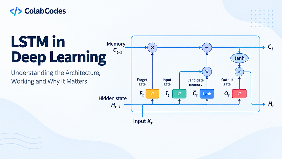
The architecture of an LSTM becomes easier to understand when it is separated into the information entering the cell, the internal memory, and the information leaving the cell.

At time step t, the LSTM receives three states or signals of interest: the current input xt, the previous hidden state ht−1, and the previous cell state ct−1. The current input contains the information presented at that position in the sequence. The previous hidden state carries the recurrent output from the preceding time step, while the cell state represents the internal state that is maintained across the sequence.

The official PyTorch formulation defines four learned transformations at each time step: the input gate it, forget gate ft, cell candidate gt, and output gate ot. These are followed by an update to the cell state and an update to the hidden state.

The standard equations are:

 it = σ ( Wii xt + bii + Whi ht-1 + bhi )

ft = σ ( Wif xt + bif + Whf ht-1 + bhf )

gt = tanh ( Wig xt + big + Whg ht-1 + bhg )

ot = σ ( Wio xt + bio + Who ht-1 + bho )

ct = ft ⊙ ct-1 + it ⊙ gt

ht = ot ⊙ tanh ( ct )

These are the standard equations documented for torch.nn.LSTM. PyTorch defines ht as the hidden state and ct as the cell state, while it, ft, gt, and ot correspond to the input, forget, cell, and output components respectively. The symbol σ denotes the sigmoid function and ⊙ denotes element-wise multiplication.

Although these equations are mathematically compact, they represent a carefully ordered information-flow mechanism.

1. The Input ( xt )

The current input xt is the information presented to the LSTM at the current position in the sequence. Depending on the task, this may represent a feature vector, an embedding, a sensor observation, or another sequential representation.

The LSTM does not process this input in isolation. It combines the current input with the previous hidden state. This allows the current computation to depend both on what is being observed now and on the representation generated from earlier parts of the sequence. PyTorch's formulation explicitly uses both xt and ht-1 when computing the recurrent transformations.

2. The Cell State ( ct )

The cell state ct is the central memory component of the LSTM architecture. Colah's widely used technical explanation describes the cell state as a relatively direct pathway running through the recurrent chain, with gates controlling what information is removed from or added to that pathway.

This is one of the most important architectural differences between an LSTM and a basic RNN. Instead of forcing all information to pass through repeated nonlinear transformations of a single hidden representation, the LSTM explicitly separates persistent cell-state information from the hidden state used for recurrent output.

The cell-state update combines two operations: retention of some portion of the previous state and addition of selected candidate information. This is precisely what the standard cell-state equation captures.

The structure is:

ct = ft ⊙ ct-1 + it ⊙ gt

Here, the forget gate determines how strongly the previous cell state contributes to the new state, while the input gate determines how strongly the candidate information contributes.

This additive update is particularly important for understanding why LSTM was developed. The original LSTM work focused on maintaining error flow over long intervals, while later analyses and implementations established the gated cell-state mechanism as the practical structure used for managing long-term information.

The Three Gates of an LSTM

The gates are the control mechanisms of the LSTM. They are learned functions rather than manually programmed rules. Each gate uses a sigmoid transformation, producing values between zero and one. Colah's explanation describes these values as controlling how much information is allowed to pass through each gating operation.

The three standard gates are the forget gate, input gate, and output gate.

1. Forget Gate

The forget gate determines how much of the previous cell state should be retained when the LSTM moves to the next time step. It is calculated from the current input and previous hidden state and produces a vector of gating values.

Its role is represented mathematically by:

ft = σ ( Wif xt + bif + Whf ht-1 + bhf )

The important point is that the forget gate does not make a single all-or-nothing decision for the entire memory. It produces a vector, allowing different components of the cell state to be retained to different degrees. A value closer to one allows more of the corresponding component of the previous state to remain, while a value closer to zero suppresses it.

Historically, the forget gate was not part of Hochreiter and Schmidhuber's original 1997 formulation. Gers, Schmidhuber, and Cummins introduced the adaptive forget gate in 2000 after identifying a limitation in LSTM when processing continual input streams without explicit sequence boundaries. Their work showed that a learnable forget mechanism could allow the cell to reset its internal state at appropriate times.

That later addition is the basis of the forget-gate mechanism found in the standard LSTM formulation used today.

2. Input Gate ( it )

The input gate controls the amount of newly generated information that can be incorporated into the cell state. Instead of immediately allowing all information from the current input to modify memory, the LSTM first calculates a gating vector that determines which components of a candidate update should be admitted. The corresponding equation is:

it = σ ( Wii xt + bii + Whi ht-1 + bhi )

The input gate works alongside the candidate cell representation. The candidate, represented as gt in PyTorch's notation, is produced using a hyperbolic tangent transformation. It represents potential new content for the cell state, but the input gate determines how much of that candidate is actually incorporated.

This distinction is important. The candidate is not equivalent to “the new memory” by itself. It is a proposed state update, while the input gate controls the extent to which that proposal influences the actual cell state.

3. Output Gate ( ot )

Once the new cell state has been calculated, the LSTM still needs to determine how much of that internal state should be exposed as the current hidden state.

That role belongs to the output gate:

ot = σ ( Wio xt + bio + Who ht-1 + bho )

The hidden state is then obtained by applying a hyperbolic tangent transformation to the cell state and modulating the result using the output gate:

ht = ot  ⊙ tanh ( ct )

These equations are part of the standard formulation documented by PyTorch.

The distinction between ct and ht is fundamental. The cell state represents the internal state carried by the memory mechanism, while the hidden state is the recurrent output produced at the current time step. PyTorch explicitly exposes both as separate states and returns them separately from an LSTM layer.

How an LSTM Works Step by Step

The actual operation of an LSTM can now be understood as a sequence of controlled memory updates. At the beginning of a time step, the network receives the current input together with the previous hidden and cell states. It first computes the input, forget, candidate, and output components from the current input and previous hidden state.

The forget gate determines which portions of the previous cell state remain relevant. At the same time, the input gate identifies the portions of the candidate update that can influence the memory. The cell-state equation then combines retained historical information with selected new information.

This means the LSTM does not simply overwrite memory at each step. Instead, the previous state and proposed update are combined in a controlled manner. Some information can persist, some can be weakened, and some new information can be introduced.

After the cell state has been updated, the output gate controls which aspects of the current memory become part of the hidden state. The resulting hidden state is then passed forward and can be used by the next time step, the next LSTM layer, or a downstream prediction layer. The sequence therefore forms a recurrent chain .i.e. at time step t, the LSTM takes xt, ht-1, and ct-1 as inputs and produces the updated ht and ct:

( xt , ht-1 , ct-1 ) → ( ht , ct )

with the same learned LSTM transformation repeatedly applied at each position. This repeated application allows an LSTM to build a representation that evolves as more of the sequence becomes available.

The overall process at each time step can therefore be summarized as:

• Receive the current input (xt), previous hidden state (ht-1), and previous cell state (ct-1).

• Compute the input gate, forget gate, cell candidate, and output gate.

• Use the forget gate to regulate information retained from (ct-1).

• Use the input gate to regulate newly generated candidate information.

• Update the cell state (ct).

• Use the output gate to regulate the information exposed through (ht).

• Pass (ht) and (ct) to the next time step.

The recurrent formulation is consistent with the broader description of RNNs, where the same parameters are shared across different positions in a sequence. As a result, an LSTM repeatedly applies the same learned transformation at each time step, while its internal states are updated according to the information encountered at each position in the sequence.

LSTM vs RNN vs GRU

Traditional RNNs are effective for processing sequential data, but they can struggle to learn dependencies across long sequences because gradients may become very small or very large during training. LSTM was introduced to address this long-term dependency problem through a more controlled memory mechanism. GRU was later developed as a simpler gated recurrent architecture, aiming to retain the benefits of LSTM while using fewer components.

Feature	RNN	LSTM	GRU
Full name	Recurrent Neural Network	Long Short-Term Memory	Gated Recurrent Unit
Basic structure	Recurrent hidden state	Hidden state + cell state	Hidden state
Main purpose	Sequence modeling	Learning short- and long-term dependencies	Efficient sequence modeling with gating
Gates	None	Input, forget, output	Update, reset
Separate cell state	No	Yes	No
Long-term dependency handling	Limited	Strong	Strong
Memory control	Through recurrent hidden state	Through cell state and gates	Through gated hidden-state updates
Vanishing-gradient resistance	Low	High	High
Parameter count	Lowest	Highest	Lower than LSTM
Computational complexity	Lower	Higher	Lower than LSTM
Training speed	Generally faster	Generally slower	Generally faster than LSTM
Architecture complexity	Simple	More complex	Simpler than LSTM
Typical use	Basic sequence tasks	Complex long-sequence dependencies	Sequence tasks where efficiency matters

The key distinction is that RNN provides the basic recurrent mechanism, LSTM adds explicit memory and three gates for more controlled information flow, while GRU simplifies this idea by combining memory and gating into a more compact architecture.

LSTM Implementation in Python

Long Short-Term Memory (LSTM) networks can be implemented in Python using deep learning frameworks such as TensorFlow and Keras. In practice, the implementation involves preparing sequential data, arranging it into the input format expected by an LSTM layer, defining the network architecture, training the model, and using the trained model to generate predictions.

For this implementation, we use Keras, which provides a high-level interface for building recurrent neural networks. The LSTM layer can process sequential inputs and maintain information across time steps, while a Dense layer can be used to transform the final LSTM representation into the required output.

Importing the Required Libraries

The first step is to import the libraries required for creating and training the model.

import numpy as np
import tensorflow as tf
from tensorflow.keras.models import Sequential
from tensorflow.keras.layers import LSTM, Dense

NumPy is used for numerical operations and handling the input data, while TensorFlow and Keras provide the components required to construct and train the LSTM network. The Sequential model allows layers to be stacked in order, and the LSTM and Dense classes are used to define the network.

Preparing Sequential Data

LSTM networks expect their input to represent a sequence. Keras LSTM layers generally receive input in the form:

(samples, time steps, features)

Here, samples represents the number of sequences in the dataset, time steps represents the number of observations within each sequence, and features represents the number of variables available at each time step.

For example, consider a simple sequence in which the model uses three previous values to predict the next value:

X = np.array([
    [1, 2, 3],
    [2, 3, 4],
    [3, 4, 5],
    [4, 5, 6],
    [5, 6, 7]
])

y = np.array([4, 5, 6, 7, 8])

Each row in X represents a sequence of three observations, while y contains the corresponding target values.

The data must be reshaped into three dimensions before it can be passed to an LSTM layer. Since there is one feature at each time step, the data can be reshaped as follows:

X = X.reshape((X.shape[0], X.shape[1], 1))

The resulting shape is:

(5, 3, 1)

This means there are five training samples, three time steps per sample, and one feature at each time step.

The distinction between time steps and features is important when working with LSTMs. For a univariate time series, each time step may contain a single value, while a multivariate sequence can contain several features at every time step.

Building the LSTM Model

Once the input data has been prepared, an LSTM model can be created using Keras:

model = Sequential([
    LSTM(50, input_shape=(3, 1)),
    Dense(1)
])

The LSTM(50) layer contains 50 LSTM units. The input_shape specifies that every input sequence contains three time steps and one feature per time step.

The Dense(1) layer produces a single output value. This configuration is commonly used for regression-style sequence prediction, where the objective is to predict one numerical value from the input sequence.

The model can be summarized using:

model.summary()

This displays information about the layers, output shapes, and number of trainable parameters in the network.

Compiling the Model

Before training, the model needs to be compiled. This step specifies the loss function and optimizer used during training.

model.compile(
    optimizer="adam",
    loss="mse"
)

Here, the Adam optimizer is used to update the model's trainable parameters, while mean squared error (mse) is used as the loss function.

The choice of loss function depends on the prediction task. Mean squared error is suitable for this numerical prediction example, but classification problems generally require an appropriate classification loss instead.

Training the LSTM

The model can now be trained using the prepared sequences and target values:

model.fit(
    X,
    y,
    epochs=100,
    batch_size=1,
    verbose=1
)

Output:
Epoch 1/100
5/5 ━━━━━━━━━━━━━━━━━━━━ 1s 8ms/step - loss: 40.5555
Epoch 2/100
5/5 ━━━━━━━━━━━━━━━━━━━━ 0s 10ms/step - loss: 36.7238
...
Epoch 100/100
5/5 ━━━━━━━━━━━━━━━━━━━━ 0s 12ms/step - loss: 0.0825

During training, the LSTM processes the sequences one time step at a time. The model calculates its prediction, compares it with the target using the specified loss function, and updates its trainable parameters through backpropagation.

The epochs parameter determines how many times the model processes the training dataset, while batch_size determines how many samples are processed before the model parameters are updated.

For larger datasets, the number of epochs and batch size should be selected based on model performance and computational requirements rather than using fixed values.

Making Predictions with the Trained LSTM

After training, the model can be used to generate predictions for new sequences.

For example:

new_data = np.array([
    [6, 7, 8]
])

new_data = new_data.reshape((new_data.shape[0], new_data.shape[1], 1))

prediction = model.predict(new_data)

print(prediction)

Output: 
Prediction: [[8.030938]]

The new input is reshaped in the same three-dimensional format used during training. The trained LSTM then processes the sequence and produces the predicted output through the final Dense layer.

Keeping the preprocessing and input structure consistent between training and prediction is essential. If the model was trained using a particular sequence length, number of features, or data transformation, new inputs should follow the same structure.

Complete LSTM Implementation

The complete implementation can be written as:

import numpy as np
import tensorflow as tf
from tensorflow.keras.models import Sequential
from tensorflow.keras.layers import LSTM, Dense

# Sequential input data
X = np.array([
    [1, 2, 3],
    [2, 3, 4],
    [3, 4, 5],
    [4, 5, 6],
    [5, 6, 7]
])

# Target values
y = np.array([4, 5, 6, 7, 8])

# Reshape input into:
# (samples, time steps, features)
X = X.reshape((X.shape[0], X.shape[1], 1))

# Build the LSTM model
model = Sequential([
    LSTM(50, input_shape=(3, 1)),
    Dense(1)
])

# Compile the model
model.compile(
    optimizer="adam",
    loss="mse"
)

# Train the model
model.fit(
    X,
    y,
    epochs=100,
    batch_size=1,
    verbose=1
)

# Prepare new sequence
new_data = np.array([[6, 7, 8]])
new_data = new_data.reshape((1, 3, 1))

# Generate prediction
prediction = model.predict(new_data)

print("Prediction:", prediction)

This example demonstrates the basic workflow for implementing an LSTM in Python: sequence preparation, reshaping, model construction, compilation, training, and prediction. In a real-world application, the same workflow can be extended to larger datasets and more complex architectures.

Conclusion

LSTMs established an important idea in sequence modeling: a recurrent network can learn to control the persistence of information instead of treating every time step as an isolated update. The combination of a persistent cell state and gated information flow gives the model a practical mechanism for carrying relevant information across long sequences while limiting the influence of information that is no longer useful. This makes LSTM a foundational architecture for understanding how neural networks can model temporal dependencies.

LSTMs also provide a natural starting point for exploring more advanced sequence models. Their limitations in computational efficiency and sequential processing eventually motivated the development and widespread adoption of architectures such as attention mechanisms and Transformers, which approach long-range dependencies in a fundamentally different way. Understanding how LSTMs manage memory and information flow therefore provides useful groundwork for understanding why modern sequence architectures evolved beyond recurrent networks.