Choosing the Right Loss Function for Machine Learning Problems

Selecting the correct loss function is one of the most critical architecture decisions in machine learning. At its core, a loss function converts the abstract goal of "making good predictions" into a precise, mathematically solvable optimization problem. It defines how a model quantifies the divergence between its predictions and ground-truth targets.

During training, an optimization algorithm attempts to minimize this loss, systematically adjusting model weights and biases to reduce prediction errors.

However, choosing an objective function is not simply a matter of grabbing a default formula from a library. Machine learning problems feature diverse output structures, error profiles, and operational requirements:

• Continuous regression tasks need loss functions that respond predictably to outliers.

• Classification models require objectives built around probability distributions and class boundaries.

• Deep learning systems depend heavily on loss functions with well-behaved gradients to avoid vanishing or exploding gradient problems.

In this guide, we will explore the mathematical mechanics, optimization behaviors, trade-offs, and practical considerations behind commonly used loss functions. For regression, we will cover Mean Squared Error (MSE), Mean Absolute Error (MAE), Mean Squared Logarithmic Error (MSLE), and Huber Loss, focusing on how each function responds to prediction errors and outliers.

For classification, we will examine Binary Cross-Entropy (Log Loss), Categorical Cross-Entropy, Sparse Categorical Cross-Entropy, Hinge Loss, and Focal Loss, along with the situations where each is most appropriate. We will also compare these loss functions to understand how their different mathematical behaviors influence model training and help determine the right choice for a given machine learning problem.

Mathematical Foundations of Loss Functions

Loss Function vs. Cost Function vs. Objective Function

While these terms are frequently used interchangeably in practice, they maintain distinct mathematical definitions:

1. Loss Function L ( y , ŷ ) : Measures the error on a single training sample (y represents the true value; ŷ represents the model’s prediction).

2. Cost Function J ( θ ) : The average loss aggregated across an entire dataset of n samples, evaluated as a function of the model’s parameters θ:

3. Objective Function: The overall function being minimized or maximized during training. This often includes the cost function alongside supplementary penalty terms like regularization parameters:

The Optimization Loop and Gradient Mechanics

For models optimized using gradient descent variants (e.g., SGD, Adam, RMSprop), parameter updates rely directly on the partial derivatives of the cost function with respect to each trainable parameter θ:

Where:

• η is the learning rate.

• ∇θ ​J (θ) is the gradient vector of partial derivatives ∂J​/∂θj.

The mathematical shape of a loss function determines the landscape of the optimization space. Smooth loss surfaces with useful gradients generally make gradient-based optimization more stable and efficient. In contrast, flat regions, sharp changes, or poorly conditioned surfaces can make optimization slower or more difficult.

A fundamental distinction exists between a training loss function and an evaluation metric. Although both are used to assess model performance, they serve different purposes during the machine learning workflow.

Metric Type	Primary Role	Key Requirements	Example
Loss Function	Guides the optimization algorithm during model training and parameter updates.	Must provide useful gradients or sub-gradients for optimization.	Binary Cross-Entropy
Evaluation Metric	Measures model performance against a task-specific objective.	Should meaningfully represent the quality of the model's predictions; differentiability is not required.	Accuracy, F1-Score, ROC-AUC

The distinction is important because the metric that best describes model performance is not necessarily the best function to optimize during training. For example, accuracy is highly intuitive for classification, but directly optimizing accuracy is generally unsuitable for gradient-based learning because accuracy changes discretely rather than providing a smooth gradient signal.

Loss Functions For Regression Based ML Problems

MSE, MAE, Mean Squared Logarithmic Error (MSLE): & Huber Loss

Regression problems predict continuous numerical values such as house prices, temperature, demand, revenue, or a customer's lifetime value. The loss function determines how the model measures the difference between its predictions and the actual target values. This choice is important because different loss functions penalize errors differently: some strongly punish large mistakes, some are more resistant to outliers, and others focus on relative rather than absolute differences.

For regression, the most commonly used loss functions include Mean Squared Error (MSE), Mean Absolute Error (MAE), Mean Squared Logarithmic Error (MSLE), and Huber Loss. Log Loss, despite sometimes appearing in lists of common machine learning losses, is fundamentally a classification loss rather than a standard regression loss. Understanding this distinction is important because the mathematical behavior of each loss function directly affects what the model learns to prioritize.

Mean Squared Error (MSE)

Mean Squared Error is one of the most widely used loss functions for regression. It measures the average squared difference between the actual target values and the predictions made by the model. Because the error is squared, larger mistakes receive disproportionately greater penalties than smaller mistakes.

For a dataset containing (n) observations, the Mean Squared Error is defined as:

The squaring operation is the defining characteristic of MSE. An error of (2) contributes (4) to the loss, while an error of (10) contributes (100). Consequently, a few very large errors can dominate the overall objective. This makes MSE particularly useful when large prediction errors are significantly more undesirable than small errors.

When the target variable contains extreme observations that are genuine and important, the sensitive nature of MSE can be desirable. However, when large errors are caused by noisy measurements, data-entry problems, or unusual observations that should not dominate training, MSE may produce an undesirable model. In such cases, a more robust loss such as MAE or Huber Loss can be preferable.

Mean Absolute Error (MAE)

Mean Absolute Error takes a fundamentally different approach to measuring regression error. Instead of squaring the residual, MAE takes its absolute value. As a result, the contribution of an error increases linearly rather than quadratically.

Across (n) observations, the objective is defined as:

MAE = ( 1/n ) Σ | yᵢ − ŷᵢ |

The absolute value ensures that positive and negative errors contribute equally to the loss while preventing them from cancelling each other out. An error of (2) contributes (2), while an error of (10) contributes (10). Unlike MSE, the larger error is not amplified by squaring.

This makes MAE considerably more robust to outliers. A small number of extreme observations cannot dominate the objective as easily as they can under MSE. For datasets containing noisy observations or heavy-tailed target distributions, this property can make MAE a more appropriate objective.

Mean Squared Logarithmic Error (MSLE)

Mean Squared Logarithmic Error is a regression loss designed for situations where the relative difference between predictions and actual values is more important than their raw numerical difference. Instead of directly comparing (y) and (\hat{y}), MSLE first applies a logarithmic transformation to both values. The complete dataset objective is:

The addition of (1) inside the logarithm allows the transformation to be defined when the target value is zero. The logarithmic transformation compresses large numerical values, reducing the influence of scale and making the loss more sensitive to relative differences.

MSLE tends to treat underprediction and overprediction in terms of proportional differences rather than simply absolute differences. A prediction that is twice the actual value can be considered more similar in severity to a prediction that is half the actual value than their raw numerical errors might suggest.

The logarithmic transformation also reduces the influence of very large target values. This can be useful for quantities such as sales, population, transaction volume, or other non-negative variables with strongly skewed distributions. However, MSLE has an important constraint: the standard formulation requires non-negative target and prediction values because the logarithm is not defined for values less than (-1), and practical implementations generally require non-negative regression targets and predictions.

Consequently, MSLE is not a good general-purpose loss for regression problems containing negative target values.

Huber Loss

Huber Loss combines characteristics of MSE and MAE. For small prediction errors, it behaves like MSE, providing a smooth quadratic penalty. For large errors, it transitions to an MAE-like linear penalty, reducing the influence of extreme observations.

This makes Huber Loss particularly useful when a regression dataset contains some outliers but we still want the smooth optimization behavior of squared error for ordinary observations. For a residual e = y − ŷ, Huber Loss is defined as:

L ( e ) = ½ e² , if | e | ≤ δ

L ( e ) = δ ( | e | − ½ δ ), if | e | > δ

where:

• y is the true value

• ŷ is the predicted value

• e is the prediction error

• δ controls the transition point between quadratic and linear behavior

For small residuals, the gradient grows with the magnitude of the error, just as it does with MSE. Once the residual exceeds the threshold, however, the gradient is capped at a magnitude determined by δ. Extremely large errors therefore cannot produce arbitrarily large gradients. This gives Huber Loss a useful middle ground between MSE and MAE. MSE provides strong sensitivity to large errors but is highly affected by outliers. MAE is robust to outliers but has a less smooth optimization landscape. Huber Loss attempts to retain the smooth behavior of MSE around the optimum while limiting the influence of extreme residuals.

In practice, Huber Loss is often a strong choice when the dataset contains occasional outliers but the model should still pay meaningful attention to large, legitimate errors. The value of δ controls how aggressively the loss treats observations as outliers, making it an important hyperparameter when using Huber Loss.

Comparing the Regression Loss Functions

MSE, MAE, MSLE, and Huber Loss all measure prediction error, but they emphasize different aspects of regression performance. MSE heavily penalizes large errors because the residual is squared, making it suitable when large mistakes should have a strong influence on model training. MAE applies a linear penalty, making it less sensitive to outliers and often more robust when the dataset contains extreme observations.

MSLE takes a different approach by applying a logarithmic transformation before calculating the squared error. This makes it useful when relative differences are more important than absolute differences, particularly for non-negative targets with a wide range of values. It also reduces the influence of very large target values compared with MSE. However, its use is more specialized because the target and predictions must satisfy the requirements of the logarithmic transformation.

Huber Loss provides a middle ground between MSE and MAE. It behaves like MSE for small errors, preserving smooth optimization around accurate predictions, but switches to a linear penalty for sufficiently large errors, reducing the influence of outliers. The choice ultimately depends on the characteristics of the regression problem: MSE for strong large-error penalties, MAE for robustness, MSLE for relative-error-oriented targets, and Huber Loss when a balance between sensitivity and robustness is needed.

Loss Functions for Classification-Based ML Problems

Binary Cross-Entropy (Log Loss), Categorical Cross-Entropy, Sparse Categorical Cross-Entropy, Hinge Loss & Focal Loss

Classification problems predict discrete categories rather than continuous numerical values. A model may determine whether an email is spam, identify an image class, predict whether a transaction is fraudulent, or assign a document to one of several categories. In these problems, the loss function measures how closely the model's predicted probabilities or class scores correspond to the actual class labels. The choice of classification loss is important because different losses influence how strongly the model responds to incorrect predictions, confident mistakes, class imbalance, and the number of target classes.

For classification, commonly used loss functions include Binary Cross-Entropy (Log Loss), Categorical Cross-Entropy, Sparse Categorical Cross-Entropy, Hinge Loss, and Focal Loss. The appropriate choice depends primarily on the structure of the classification problem and the type of output produced by the model. Binary Cross-Entropy is commonly used for binary classification, Cross-Entropy variants are widely used for multiclass problems, Hinge Loss is associated with margin-based classification, and Focal Loss is particularly useful when difficult or minority-class examples need greater attention during training.

Binary Cross-Entropy (Log Loss)

Binary Cross-Entropy, commonly called Log Loss, is one of the standard loss functions for binary classification. It is designed for models that produce a probability between 0 and 1 representing the likelihood that an observation belongs to the positive class. Unlike regression losses that compare continuous numerical values directly, Binary Cross-Entropy evaluates the quality of the predicted probability. Binary Cross-Entropy is defined as:

where y is the actual binary label and ŷ is the predicted probability of the positive class. The loss becomes small when the model assigns a high probability to the correct class and becomes very large when the model is confidently wrong. The logarithmic penalty is important because it heavily penalizes confident incorrect predictions. A model that predicts the wrong class with high confidence receives a substantially larger loss than a model that makes the same incorrect classification with low confidence.

This encourages the model not only to classify observations correctly but also to produce probabilities that better reflect its confidence. Binary Cross-Entropy is commonly used with logistic regression and neural networks for binary classification. In neural networks, it is typically paired with a sigmoid output so that the model produces a probability between 0 and 1.

Categorical Cross-Entropy

Categorical Cross-Entropy extends the idea of Binary Cross-Entropy to multiclass classification problems. It is used when an observation belongs to exactly one class among multiple possible classes and the model produces a probability distribution across those classes. It measures the difference between the true class distribution and the probability distribution predicted by the model. When the target is one-hot encoded, the correct class has a value of 1, while all other classes have a value of 0. As a result, the loss primarily depends on the probability assigned to the correct class, with lower probabilities producing higher penalties. It can therefore be viewed as:

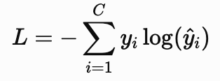
Categorical Cross-Entropy is commonly paired with a softmax output layer. The softmax function converts the model's raw class scores, or logits, into probabilities whose values sum to (1). This makes the loss particularly suitable for mutually exclusive multiclass classification tasks.

Sparse Categorical Cross-Entropy

Sparse Categorical Cross-Entropy uses the same underlying mathematical principle as Categorical Cross-Entropy but represents the target differently. Instead of requiring one-hot encoded labels, each observation is represented using a single integer corresponding to its correct class.

The loss behaves in the same fundamental way as Categorical Cross-Entropy: assigning a high probability to the correct class produces a low loss, while assigning a low probability produces a high loss. The primary difference between Categorical Cross-Entropy and Sparse Categorical Cross-Entropy is therefore the representation of the target labels rather than the underlying learning objective. Categorical Cross-Entropy uses one-hot encoded targets, while Sparse Categorical Cross-Entropy uses integer class labels.

This distinction becomes particularly useful when working with datasets containing a large number of classes. Integer labels can be more memory-efficient than explicitly storing a one-hot vector for every observation. In practical machine learning frameworks, Sparse Categorical Cross-Entropy is therefore convenient when the training data already contains integer-encoded class labels.

Hinge Loss

Hinge Loss is a margin-based classification loss most closely associated with Support Vector Machines (SVMs). Instead of directly optimizing predicted probabilities, Hinge Loss encourages the model to assign the correct class a sufficiently large score relative to the incorrect class. For binary classification with labels represented as y taking values one or negative one, the Hinge Loss for one observation is:

Here, f(x) represents the model's decision score. The loss becomes zero when the prediction is not only correct but sufficiently far from the decision boundary. If the prediction is correct but falls within the desired margin, the model still receives a non-zero penalty.

This margin-based behavior is the defining characteristic of Hinge Loss. The objective is not simply to classify observations correctly but to create a sufficiently large separation between classes. This is particularly important in SVMs, where the decision boundary is determined by maximizing the margin between classes.

For an observation that is correctly classified with a sufficiently large margin, y f(x) greater then or equal to 1, the loss is zero:

When the margin is violated, the loss increases according to the degree of that violation. This makes Hinge Loss fundamentally different from Cross-Entropy, which is naturally interpreted in terms of predicted probabilities.

Hinge Loss is particularly appropriate for margin-based classifiers and situations where the separation between classes is important. It is less suitable when calibrated probability estimates are required because the output score itself is not necessarily a probability.

Focal Loss

Focal Loss was designed to address a common challenge in classification: class imbalance. In highly imbalanced datasets, the majority class may contain a large number of examples that are relatively easy for the model to classify. Standard Cross-Entropy can become dominated by these easy examples, potentially reducing the attention given to difficult or minority-class observations.

Focal Loss modifies the standard Cross-Entropy objective by introducing a factor that reduces the contribution of well-classified examples. For a binary classification problem, it can be written as:

Here, pₜ represents the probability assigned to the correct class, α is a weighting factor used to address class imbalance, and γ controls how strongly the loss focuses on difficult examples.

The term ( 1 - pₜ )ᵞ is the key addition. When an example is classified correctly with high confidence, pₜ approaches 1, causing this factor to become small. Consequently, easy examples contribute less to the overall loss. When the model struggles with an observation and pₜ is small, the focusing factor becomes larger, increasing the relative importance of that example.

The focusing parameter ᵞ therefore controls how aggressively the loss down-weights easy examples. When γ, the focusing factor becomes (1), and Focal Loss reduces to a weighted form of Cross-Entropy:

As γ increases, the contribution of confidently classified observations is reduced more strongly. This makes Focal Loss particularly useful for heavily imbalanced classification tasks such as object detection, fraud detection, and other problems where difficult minority-class examples are more important than large numbers of easy majority-class examples.

Comparing the Classification Loss Functions

Binary Cross-Entropy, Categorical Cross-Entropy, Sparse Categorical Cross-Entropy, Hinge Loss, and Focal Loss are designed for different classification settings. Binary Cross-Entropy is generally appropriate when there are two classes and the model produces a probability for the positive class. Categorical Cross-Entropy is commonly used for multiclass classification with one-hot encoded targets, while Sparse Categorical Cross-Entropy is used when the same multiclass targets are represented as integer class labels.

Hinge Loss takes a different approach by focusing on the margin between classes rather than directly optimizing probabilities, making it particularly relevant to SVM-style classifiers. Focal Loss builds on Cross-Entropy by reducing the contribution of easy examples and placing greater emphasis on difficult observations, making it especially useful for imbalanced classification datasets.

The choice of classification loss should therefore be based on the structure of the prediction problem and the behavior required from the model. Binary Cross-Entropy is a strong default for binary probabilistic classification, Cross-Entropy variants are widely used for multiclass neural networks, Hinge Loss is appropriate for margin-based classification, and Focal Loss becomes valuable when class imbalance causes standard Cross-Entropy to focus too heavily on easy majority-class examples.

Conclusion

The loss function ultimately defines what a machine learning model is being optimized to achieve. Choosing it is therefore not just a technical implementation detail, but a decision about how prediction errors should be treated. A well-chosen loss function aligns the training objective with the behavior we expect from the final model.

The key is to look beyond simply asking which loss function is most commonly used. The nature of the target variable, the distribution of the data, the presence of outliers or class imbalance, and the practical consequences of different errors should all influence the decision. Once these factors are understood, selecting a loss function becomes a deliberate modeling decision rather than a default choice.

In the end, there is no universally “best” loss function. The right choice is the one that best represents the objective of the machine learning problem and encourages the model to learn the behavior that matters in practice. Understanding that relationship between the problem, the loss, and the resulting optimization process is what turns loss-function selection from a formula on paper into an important part of building reliable machine learning systems.