

Entropy Loss Functions in Machine Learning: Cross-Entropy, Binary Cross-Entropy, and Beyond
Entropy-based loss functions form the mathematical foundation of modern classification models, enabling machine learning algorithms to learn from probability distributions rather than simple prediction errors. Rooted in information theory, these loss functions provide a principled way to quantify uncertainty, evaluate prediction quality, and optimize model parameters. Their effectiveness has made them the default choice for training a wide range of models, from logistic regression and convolutional neural networks to today's transformer architectures and large language models.
In this blog, we explain the theoretical foundations of entropy and its role in information theory before demonstrating how it naturally leads to Cross-Entropy Loss. We then explore Binary Cross-Entropy, Categorical Cross-Entropy, and several related entropy-based loss functions, including Sparse Categorical Cross-Entropy, KL Divergence, Label Smoothing, and Focal Loss. Along the way, we discuss their mathematical formulations, practical applications, and intuitive interpretations, followed by Python implementations that illustrate how these concepts are applied in real-world machine learning workflows.

Foundations of Entropy in Information Theory
Before we can understand entropy-based loss functions used in machine learning, we must first understand the concept of entropy itself. Entropy originated in information theory through the pioneering work of Claude Shannon in 1948. It provides a mathematical way to quantify uncertainty or, equivalently, the amount of information contained in an event. Nearly every modern classification loss function, including cross-entropy and binary cross-entropy, traces its theoretical foundation back to this single concept.
In everyday life, information is valuable because it reduces uncertainty. Consider predicting tomorrow's weather. If it rains every single day in a particular region, learning that tomorrow will also be rainy provides almost no new information because the outcome was already expected. On the other hand, if the weather is equally likely to be sunny, rainy, snowy, or windy, discovering tomorrow's forecast conveys much more information because the prediction was uncertain.
Information theory formalizes this intuition by assigning greater information content to rare events and less information content to common ones. The information obtained when an event with probability p occurs is defined as

where:
I ( x ) is the information content of event x,
p ( x ) is the probability of the event,
The logarithm is typically base 2 (bits) or the natural logarithm (nats).
This equation captures an intuitive principle:
Highly probable events carry little information.
Rare events carry much more information.
For example,
Event Probability | Information Content |
1.0 | 0 |
0.5 | 1 bit |
0.25 | 2 bits |
0.125 | 3 bits |
Shannon Entropy
While information content measures the surprise associated with a single event, Shannon entropy measures the average uncertainty across an entire probability distribution.
For a discrete random variable X with possible outcomes x1, x2… xn, Shannon entropy is defined as
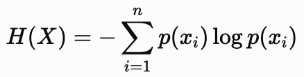
where:
H ( X ) is the entropy,
p ( xi ) is the probability of outcome xi,
The summation covers every possible outcome.
Entropy can be interpreted as the expected amount of information obtained after observing the outcome of a random variable. If every outcome is equally likely, uncertainty is high, resulting in high entropy. If one outcome dominates, uncertainty decreases and entropy becomes smaller.
We can compute it directly using NumPy by applying the entropy equation.
import numpy as np

def shannon_entropy(probabilities):
    probabilities = np.array(probabilities)
    probabilities = probabilities[probabilities > 0]
    return -np.sum(probabilities * np.log2(probabilities))

p = [0.25, 0.25, 0.25, 0.25]
entropy = shannon_entropy(p)

print(f"Shannon Entropy: {entropy:.4f} bits")

Output:
Shannon Entropy: 2.0000 bits
Entropy as a Measure of Unpredictability
Entropy is often described as a measure of randomness or unpredictability. The more difficult it is to predict an outcome before observing it, the higher the entropy.
Imagine rolling two different dice.
The first die is perfectly fair.
Outcome | Probability |
1 | 1/6 |
2 | 1/6 |
3 | 1/6 |
4 | 1/6 |
5 | 1/6 |
6 | 1/6 |
Every outcome is equally likely, making the result highly unpredictable. Consequently, this distribution has high entropy.
Now consider a loaded die.
Outcome | Probability |
1 | 0.90 |
2 | 0.02 |
3 | 0.02 |
4 | 0.02 |
5 | 0.02 |
6 | 0.02 |
Because the die lands on 1 almost every time, the outcome is highly predictable. The uncertainty is much lower, leading to low entropy.
In general:
High entropy indicates greater uncertainty and less confidence in predicting outcomes.
Low entropy indicates greater certainty and more predictable outcomes.
Entropy therefore provides a numerical measure of how difficult it is to make accurate predictions before observing the true result.
Why Entropy Matters in Machine Learning
Entropy serves as the mathematical foundation for many of the loss functions used to train modern machine learning models. Classification algorithms do not simply predict labels they estimate probability distributions over possible classes. The quality of these probability estimates determines how effectively a model learns.
Suppose a neural network predicts the probabilities [0.60, 0.40], while the true class is the second one. Although the prediction is close, the model has assigned a higher probability to the wrong class. During training, we need a way to measure how far this predicted distribution is from the desired distribution. This is precisely where entropy-based loss functions come into play.
Cross-entropy extends the concept of Shannon entropy by comparing two probability distributions: the model's predicted distribution and the true distribution represented by the training labels. The resulting loss quantifies prediction error in a mathematically principled way, allowing optimization algorithms such as gradient descent to iteratively improve the model.
Because of this property, entropy forms the theoretical backbone of numerous machine learning algorithms, including logistic regression, neural networks, convolutional neural networks (CNNs), recurrent neural networks (RNNs), transformers, large language models (LLMs), and many other probabilistic classifiers. Understanding entropy therefore provides the essential foundation for understanding why cross-entropy and binary cross-entropy have become the standard loss functions for modern classification tasks.
From Entropy to Cross-Entropy Loss
After understanding entropy as a measure of uncertainty, the next question naturally arises: how can we use this concept to train machine learning models? While Shannon entropy quantifies the uncertainty within a single probability distribution, machine learning requires something more practical. During training, a model generates its own probability distribution, which must be compared against the true distribution represented by the training labels. This comparison is performed using the cross-entropy loss function, one of the most widely used objective functions in modern classification algorithms.
Cross-entropy extends Shannon's concept by measuring the discrepancy between what the model predicts and what the data actually tells us. By minimizing this discrepancy, learning algorithms gradually adjust their parameters to produce increasingly accurate predictions.
A classification model does not simply predict a class label; instead, it estimates the probability that an input belongs to each possible class.
For example, a model classifying an image of an animal might produce y^=[0.75, 0.20, 0.05]
indicating a 75% probability for class 1, 20% for class 2, and 5% for class 3.
Suppose the correct label is y=[1, 0, 0]
Although the prediction is correct, it is not perfect because the model still assigns probabilities to the incorrect classes. During training, we require a mathematical function that tells us how good or bad these predicted probabilities are.
A useful loss function should satisfy several properties:
Produce a small value when predictions closely match the true labels.
Produce a large value for incorrect or overconfident predictions.
Be continuous and differentiable so that optimization algorithms such as gradient descent can update the model parameters efficiently.
Cross-entropy satisfies all these requirements, making it the standard loss function for classification problems.
Deriving Cross-Entropy from Shannon Entropy
Recall that Shannon entropy measures the average uncertainty within a probability distribution:

where P represents the true probability distribution. In supervised learning, however, we are not interested in measuring the uncertainty of the true distribution alone. Instead, we want to evaluate how well another distribution, the model's predicted distribution matches it. Let
P(i) denote the true probability,
Q(i) denote the probability predicted by the model.
Replacing the logarithm of the true distribution with the logarithm of the predicted distribution yields the cross-entropy:

This simple modification transforms entropy from a measure of uncertainty into a measure of prediction error. If the predicted probabilities closely resemble the true probabilities, the cross-entropy becomes small. As the predictions deviate from the truth, the loss increases.
For multi-class classification using one-hot encoded labels, only one class has a probability of 1 while all others are 0.
Suppose y = [ 0, 1, 0 ] and the model predicts y^ = [ 0.15, 0.80, 0.05 ], applying the cross-entropy equation,

all terms vanish except the correct class because the remaining entries of y are zeros and thus, L = − log ( 0.80 ) = 0.223. Now consider a poor prediction, y^ = [ 0.80, 0.15, 0.05 ]
The loss becomes L = − log ( 0.15 ) = 1.897. Although both predictions assign probabilities that sum to one, the second prediction incurs a much larger penalty because it assigns a low probability to the correct class.
This logarithmic penalty is one of the defining characteristics of cross-entropy. As the predicted probability for the correct class approaches zero, the loss grows rapidly, discouraging highly confident but incorrect predictions.
Binary Cross-Entropy for Binary Classification
While cross-entropy provides a general framework for measuring the difference between two probability distributions, many real-world machine learning problems involve only two possible outcomes. Determining whether an email is spam or not spam, diagnosing whether a patient has a disease or not, detecting fraudulent transactions, or recognizing whether an image contains a cat or not are all examples of binary classification problems.
For these tasks, the general cross-entropy equation simplifies into a specialized form known as Binary Cross-Entropy (BCE), also referred to as Log Loss. Binary cross-entropy is one of the most widely used loss functions in machine learning because it effectively measures how well a model predicts the probability of one of two mutually exclusive classes.
Binary cross-entropy evaluates how close the predicted probability is to the actual class label. Its mathematical definition is

where
y is the true label (0 or 1),
y^ is the predicted probability of the positive class.
Notice that the equation contains two terms. The first term, y log ( y^ ), is active only when the true label is 1. The second term, ( 1 − y ) log ( 1 − y^ ), is active only when the true label is 0. This elegant formulation allows a single equation to handle both positive and negative examples.
Binary cross-entropy is closely connected to maximum likelihood estimation. During training, the model attempts to maximize the probability of observing the correct labels in the training data. Minimizing the binary cross-entropy loss is mathematically equivalent to maximizing this likelihood.
In deep learning, binary cross-entropy is typically paired with a sigmoid activation function in the output layer. The sigmoid converts the model's raw output (logit) into a probability between 0 and 1, which is then compared against the true binary label using the BCE loss. Together, the sigmoid activation and binary cross-entropy form the foundation of binary classification models, enabling them to learn accurate probability estimates while maintaining stable and efficient optimization.
For binary classification problems, python allows us to implement Binary Cross-Entropy using its simplified mathematical formulation.
import numpy as np

def binary_cross_entropy(y_true, y_pred):
    epsilon = 1e-12
    y_pred = np.clip(y_pred, epsilon, 1 - epsilon)

    return -np.mean(
        y_true * np.log(y_pred) +
        (1 - y_true) * np.log(1 - y_pred)
    )

y_true = np.array([1, 0, 1, 1])
y_pred = np.array([0.9, 0.2, 0.75, 0.95])

loss = binary_cross_entropy(y_true, y_pred)

print(f"Binary Cross-Entropy: {loss:.4f}")

Output:
Binary Cross-Entropy: 0.1669
Categorical Cross-Entropy
Categorical Cross-Entropy (CCE) is the standard loss function for multi-class classification problems where each sample belongs to exactly one class. The model outputs a probability distribution over all possible classes, typically using a softmax activation function, and the loss measures how closely these predicted probabilities match the true labels.
The mathematical formulation of Categorical Cross-Entropy is
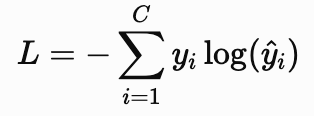
where:
C is the total number of classes,
yi is the true probability for class iii (usually one-hot encoded),
y^i is the probability predicted by the model for class iii.
Since only one entry in a one-hot encoded label equals 1, the equation simplifies to

meaning the loss depends solely on the probability assigned to the correct class. As the model assigns higher probability to the correct class, the loss decreases toward zero, while assigning low probability to the correct class results in a large penalty.
Categorical Cross-Entropy can be implemented by comparing one-hot encoded labels with the predicted probability distribution.
import numpy as np

def categorical_cross_entropy(y_true, y_pred):
    epsilon = 1e-12
    y_pred = np.clip(y_pred, epsilon, 1.0)

    return -np.sum(y_true * np.log(y_pred))

y_true = np.array([0, 0, 1, 0])
y_pred = np.array([0.05, 0.10, 0.80, 0.05])

loss = categorical_cross_entropy(y_true, y_pred)

print(f"Categorical Cross-Entropy: {loss:.4f}")

Output:
Categorical Cross-Entropy: 0.2231
Sparse Categorical Cross-Entropy
Sparse Categorical Cross-Entropy (SCCE) is mathematically equivalent to Categorical Cross-Entropy but represents the true labels differently. Instead of using one-hot encoded vectors, the labels are stored as integer class indices.
For example, One-hot encoding: [ 0, 0, 1, 0 ], Sparse representation: 2.
The underlying loss remains identical to Categorical Cross-Entropy, but sparse labels reduce memory usage and simplify data preprocessing when working with datasets containing many classes.
When labels are stored as integer class indices instead of one-hot vectors, we can compute Sparse Categorical Cross-Entropy as follows.
import numpy as np

def sparse_categorical_cross_entropy(y_true, y_pred):
    epsilon = 1e-12
    y_pred = np.clip(y_pred, epsilon, 1.0)

    return -np.log(y_pred[y_true])

y_true = 2
y_pred = np.array([0.10, 0.15, 0.70, 0.05])

loss = sparse_categorical_cross_entropy(y_true, y_pred)

print(f"Sparse Categorical Cross-Entropy: {loss:.4f}")

Output:
Sparse Categorical Cross-Entropy: 0.3567
Kullback-Leibler (KL) Divergence
Kullback-Leibler Divergence measures how one probability distribution differs from another. Unlike cross-entropy, which measures the expected information required to encode one distribution using another, KL divergence quantifies the additional information lost when the predicted distribution approximates the true distribution.
Its mathematical definition is

where:
P is the true probability distribution,
Q is the predicted probability distribution.
KL divergence is always non-negative and equals zero only when the two distributions are identical. It is widely used in probabilistic machine learning, Bayesian inference, variational autoencoders (VAEs), knowledge distillation, and reinforcement learning.
Python makes it straightforward to calculate the Kullback-Leibler (KL) Divergence between two probability distributions.
import numpy as np

def kl_divergence(p, q):
    epsilon = 1e-12

    p = np.clip(p, epsilon, 1)
    q = np.clip(q, epsilon, 1)

    return np.sum(p * np.log(p / q))

# Example
P = np.array([0.6, 0.3, 0.1])
Q = np.array([0.5, 0.4, 0.1])

kl = kl_divergence(P, Q)

print(f"KL Divergence: {kl:.4f}")

Output:
KL Divergence: 0.0231
Label Smoothing
Traditional cross-entropy assumes that the correct class has probability 1 while every other class has probability 0. Label Smoothing relaxes this assumption by assigning a small probability to the incorrect classes, preventing models from becoming excessively confident. The smoothed target distribution is defined as
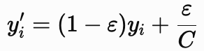
where:
ε is the smoothing factor,
C is the number of classes.
Label smoothing often improves model generalization, calibration, and robustness, particularly in large neural networks and transformer-based architectures.
We can implement Label Smoothing by redistributing a small portion of the target probability across all classes.
import numpy as np

def label_smoothing(one_hot, epsilon=0.1):
    num_classes = len(one_hot)
    return (1 - epsilon) * one_hot + epsilon / num_classes

label = np.array([0, 0, 1, 0])

smoothed = label_smoothing(label)

print(smoothed)

Output:
[0.025 0.025 0.925 0.025]
Focal Loss
In many classification tasks, such as object detection or medical diagnosis, the dataset is highly imbalanced, with far more easy examples than difficult ones. Standard cross-entropy treats every sample equally, causing the model to focus excessively on already well-classified examples. Focal Loss addresses this issue by reducing the contribution of easy samples and emphasizing difficult ones. Its mathematical formulation is

where:
pt is the predicted probability of the correct class,
γ is the focusing parameter that controls how strongly easy examples are down-weighted.
When a prediction is already highly accurate, the weighting term ( 1 − pt ) ^γ becomes very small, allowing the model to devote more learning capacity to challenging examples. Focal Loss is widely used in object detection models such as RetinaNet and other applications involving severe class imbalance.
Finally, Focal Loss can be implemented by introducing a focusing parameter that reduces the influence of easy training examples.
import numpy as np

def focal_loss(y_true, y_pred, gamma=2.0):
    epsilon = 1e-12
    y_pred = np.clip(y_pred, epsilon, 1 - epsilon)

    pt = np.where(y_true == 1, y_pred, 1 - y_pred)

    return -np.mean((1 - pt) ** gamma * np.log(pt))

y_true = np.array([1, 0, 1, 1])
y_pred = np.array([0.95, 0.30, 0.80, 0.60])

loss = focal_loss(y_true, y_pred)

print(f"Focal Loss: {loss:.4f}")

Output:
Focal Loss: 0.0307
Conclusion
Entropy-based loss functions have become the standard for classification because they do far more than measure prediction errors—they shape how a model learns. By treating learning as the task of aligning predicted probability distributions with reality, these loss functions provide a mathematically principled objective that enables stable optimization, faster convergence, and well-calibrated predictions. Their strong theoretical foundation and practical effectiveness have made them indispensable across virtually every domain of modern machine learning.
As AI systems continue to evolve, the role of entropy-based optimization remains as important as ever. From simple binary classifiers to sophisticated transformer architectures and large language models, these loss functions continue to drive learning by converting uncertainty into actionable feedback for optimization algorithms. Understanding their mathematical foundations equips practitioners with the insight to choose the appropriate loss function for a given problem, diagnose training behavior, and build models that are not only more accurate but also more reliable and robust in real-world applications.


