Logistic Regression from Scratch: Math, Intuition, and Python Implementation

Many real-world problems are not about predicting exact numbers, but about making decisions between two possibilities. For example, determining if an email is spam or not, if a tumor is malignant or benign, or if a customer will churn or stay. These are all classification problems where the output is categorical rather than continuous.

What makes logistic regression particularly important is its simplicity combined with strong mathematical grounding. It acts as a bridge between linear models and probability theory, transforming raw linear outputs into meaningful probability values between 0 and 1.

Instead of directly predicting class labels, logistic regression estimates the probability of a given input belonging to a particular class. This probabilistic interpretation makes it highly interpretable and widely used in domains like healthcare, finance, and natural language processing.

In this blog, we will build logistic regression from scratch, starting from its mathematical foundation, understanding the intuition behind the sigmoid function, cost function, gradient descent and finally implementing it step-by-step in Python without relying on high-level abstractions.

What is Logistic Regression?

Logistic regression is a supervised machine learning algorithm designed for classification problems, where the objective is to predict discrete labels instead of continuous numerical values. It is most commonly used in binary classification tasks such as spam detection, disease diagnosis, customer churn prediction, and fraud detection.

Unlike regression models that directly output a continuous value, logistic regression focuses on estimating probabilities. This means instead of saying “this is class 1,” it answers the more useful question: how likely is this input to belong to class 1?

To achieve this, the model first builds a linear relationship between the input features and the output. This step is identical in structure to linear regression and can be written as:

Here, the input vector x contains the features of a data point, w represents the learned weights that determine the importance of each feature, and bbb is the bias term that shifts the decision boundary.

At this stage, z can take any real value from negative infinity to positive infinity. However, this creates a problem. Raw linear outputs cannot be interpreted as probabilities because probabilities must always lie between 0 and 1. This is where logistic regression introduces a key transformation.

Instead of using z directly, we pass it through a function that compresses any real-valued number into a bounded range. This function is called the sigmoid function.

The sigmoid function is defined as:

This function has a very important property: no matter what value z takes, the output will always stay between 0 and 1. Large positive values of z push the output closer to 1, while large negative values push it closer to 0.

This transformation is what gives logistic regression its probabilistic interpretation. It allows us to treat the output as a probability rather than just a raw score.

By combining the linear model and the sigmoid function, we get the final hypothesis function of logistic regression:

This function represents the model’s prediction of the probability that a given input belongs to class 1. In probabilistic terms, it can be written as:

Once this probability is computed, we still need to convert it into a final decision. This is done using a threshold rule. The most commonly used threshold is 0.5, meaning that if the predicted probability is greater than or equal to 0.5, the model predicts class 1; otherwise, it predicts class 0.

This decision rule effectively splits the feature space into two regions using what is known as a decision boundary.

The Decision Boundary

After computing probabilities using the sigmoid function, logistic regression still needs a mechanism to separate one class from another. This separation is achieved using a decision boundary. The point where the prediction changes from one class to another is called the decision boundary and is given by:

This equation defines the surface that separates the feature space into different regions. In two dimensions, the decision boundary is a straight line. In three dimensions, it becomes a plane, and in higher dimensions it forms a hyperplane.

The position and orientation of this boundary depend entirely on the learned weights and bias values.

One important property of logistic regression is that it creates a linear decision boundary. This works well when classes are linearly separable, meaning they can be divided using a straight line or hyperplane. However, for highly complex datasets with non-linear structures, logistic regression may struggle unless feature engineering or transformations are applied.

The decision boundary is ultimately what allows logistic regression to perform classification. While the sigmoid function provides probabilities, the decision boundary converts those probabilities into meaningful class predictions.

The Cost Function / Log Loss

To make accurate predictions, logistic regression must learn the optimal values of the weights and bias. This requires a way to measure how good or bad the predictions are during training.

In machine learning, this measurement is performed using a cost function.

For linear regression, Mean Squared Error (MSE) is commonly used. However, MSE is not ideal for logistic regression because the sigmoid function makes the optimization landscape non-convex, which can lead to inefficient learning and local minima problems.

Instead, logistic regression uses a specialized loss function called Log Loss, also known as Binary Cross-Entropy Loss. The loss for a single training example is defined as:

This equation behaves differently depending on the true class label. If the true label is y = 1, then the loss simplifies to:

This means the model is heavily penalized when it predicts a probability close to 0 for the correct class. Similarly, if y = 0 the loss becomes:

In this case, the model receives a large penalty when it predicts probabilities close to 1 for the wrong class.

To compute the overall training error across all examples, we take the average loss over the dataset:

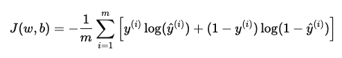
where, m is the total number of training examples.

The objective of training is to minimize this cost function by finding the best values of the parameters  and b.

One of the biggest advantages of log loss is that it creates a convex optimization problem for logistic regression, allowing gradient descent to converge efficiently toward the global minimum.

Gradient Descent Optimization

Once the cost function has been defined, the next step is to minimize it. Logistic regression achieves this using an optimization algorithm called gradient descent.

Gradient descent works by iteratively adjusting the model parameters in the direction that reduces the cost function.

The parameters of logistic regression are w and b. he objective is to find values of these parameters that minimize J(w,b).

The algorithm begins with randomly initialized weights and bias values. During each iteration, it calculates how much the cost function changes with respect to each parameter. These changes are called gradients.

The weights are updated using:

Similarly, the bias term is updated as:

where α is the learning rate, ∂J/∂w represents the gradient of the cost with respect to the weights & ∂J/∂b represents the gradient with respect to the bias.

The learning rate controls the step size during optimization. If the learning rate is too large, the algorithm may overshoot the minimum. If it is too small, training becomes very slow.

For logistic regression, the gradients are derived from the log loss function and can be written as:

and

These gradients measure the direction and magnitude of parameter updates required to reduce prediction error.

The optimization process continues iteratively until the cost function converges to a minimum value or the maximum number of iterations is reached.

Gradient descent is one of the most fundamental optimization techniques in machine learning and forms the foundation for training not only logistic regression, but also neural networks and deep learning models.

How Logistic Regression Learns

Now that we have explored the mathematical foundation of logistic regression, it becomes easier to understand how all these components work together during the training process.

During every iteration, logistic regression follows a structured sequence of operations to gradually improve its predictions. The model first computes a linear combination of the input features using the weights and bias terms. This output is then passed through the sigmoid function, which converts the raw value into a probability between 0 and 1.

Using these probabilities, the model generates predictions for each training example. The predicted values are then compared with the actual labels using the log loss cost function, which measures how far the predictions are from the true outputs.

Once the error is computed, gradient descent calculates the gradients of the cost function with respect to the model parameters. These gradients indicate the direction in which the weights and bias should be updated to reduce the prediction error.

The parameters are then updated iteratively, allowing the model to slowly move toward the optimal solution.

The complete learning cycle can be summarized as follows:

1. Compute the linear combination

2. Apply the sigmoid function

3. Generate prediction probabilities

4. Calculate the log loss

5. Compute gradients

6. Update weights and bias using gradient descent

This process repeats continuously until the cost function converges to a minimum value or the model reaches a stable solution.

In essence, logistic regression learns by repeatedly adjusting its parameters to reduce prediction error. The sigmoid function enables probability estimation, the decision boundary performs classification, the cost function evaluates prediction quality, and gradient descent optimizes the model parameters during training.

Implementing Logistic Regression from Scratch in Python

Rather than relying entirely on high-level machine learning libraries, implementing logistic regression manually provides a much deeper understanding of how the model actually learns from data. It allows us to see how the sigmoid function transforms predictions into probabilities, how the cost function measures error, and how gradient descent updates the model parameters iteratively during training.

In this implementation, we will construct every major component of logistic regression step by step. Starting from initializing the weights and bias, we will implement forward propagation, compute the binary cross-entropy loss, calculate gradients, and optimize the model using gradient descent.

To keep the focus on the learning process itself, we will primarily use NumPy for matrix operations and numerical computations, while Matplotlib will help us visualize the dataset and training behavior.

1. Importing Libraries and Creating the Dataset

The implementation begins by importing the required Python libraries for numerical computation, visualization, and dataset generation. NumPy is used for efficient matrix operations and mathematical calculations, while Matplotlib helps visualize the data distribution and model behavior. The make_classification() function from scikit-learn is used to generate a synthetic binary classification dataset.

The generated dataset contains 1000 samples with two informative features, making it easy to visualize how logistic regression separates the two classes using a decision boundary. The feature values are stored in X, while the corresponding class labels are stored in y. This dataset provides a clean foundation for understanding how logistic regression learns patterns and performs classification.

# Import Libraries
import numpy as np
import matplotlib.pyplot as plt
from sklearn.datasets import make_classification
from sklearn.model_selection import train_test_split

# Create Dataset
X, y = make_classification(
    n_samples=1000,
    n_features=2,
    n_redundant=0,
    n_informative=2,
    n_clusters_per_class=1,
    random_state=42
)

2. Splitting and Visualizing the Dataset

Before training the logistic regression model, the dataset is divided into training and testing sets using the train_test_split() function from scikit-learn. The training set is used to learn the model parameters, while the testing set helps evaluate how well the model performs on unseen data. Here, 80% of the data is allocated for training and the remaining 20% is reserved for testing.

# Split dataset into training and testing sets
X_train, X_test, y_train, y_test = train_test_split(
    X, y,
    test_size=0.2,
    random_state=42
)

The target labels are then reshaped into column vectors to ensure compatibility during matrix operations in forward propagation and gradient calculations. After preprocessing, the dataset is visualized using Matplotlib.

# Reshape labels
y_train = y_train.reshape(-1, 1)
y_test = y_test.reshape(-1, 1)

# Visualize Dataset
plt.figure(figsize=(8, 6))
plt.scatter(X[:, 0], X[:, 1], c=y, cmap='bwr')
plt.xlabel("Feature 1")
plt.ylabel("Feature 2")
plt.title("Binary Classification Dataset")
plt.show()

Since the dataset contains only two features, the data points can be plotted in a two-dimensional space, making it easier to observe how the two classes are distributed and how logistic regression will eventually learn a decision boundary to separate them.

3. Initializing Parameters and Implementing Forward Propagation

Before the learning process begins, logistic regression requires initial values for the model parameters. The number of input features is extracted from the training dataset, and the weight vector is initialized with zeros, while the bias term is set to zero. These parameters will later be updated iteratively during gradient descent as the model learns the relationship between the input features and target labels.

# Initialize Parameters
n_features = X_train.shape[1]

weights = np.zeros((n_features, 1))
bias = 0

The sigmoid function is then implemented to transform the linear output of the model into probability values between 0 and 1. Since logistic regression is fundamentally a probabilistic classification algorithm, this transformation is essential for interpreting predictions as class probabilities.

# Sigmoid Function
def sigmoid(z):
    return 1 / (1 + np.exp(-z))

Forward propagation combines these components into a single prediction pipeline. The input features are first multiplied by the weights and added to the bias term to compute the linear model output. This result is then passed through the sigmoid function, producing prediction probabilities for each training example. These probabilities represent the likelihood that a given input belongs to the positive class.

# Forward Propagation
def forward_propagation(X, weights, bias):
    linear_model = np.dot(X, weights) + bias
    predictions = sigmoid(linear_model)
    return predictions

4. Computing the Cost Function and Gradients

Once prediction probabilities are generated through forward propagation, the next step is to measure how accurate those predictions are. This is done using the binary cross-entropy loss function, also known as log loss. The cost function compares the predicted probabilities with the actual class labels and produces a numerical value representing the prediction error across the dataset.

To avoid computational issues such as taking the logarithm of zero, the predicted probabilities are clipped using a very small value epsilon. This improves numerical stability during training. The overall cost is then computed by averaging the log loss across all training examples, allowing the model to quantify how far its predictions are from the true labels.

# Compute Cost Function (Log Loss)
def compute_cost(y_true, y_pred):
    m = len(y_true)
    epsilon = 1e-15
    y_pred = np.clip(y_pred, epsilon, 1 - epsilon)
    cost = -(1 / m) * np.sum(
        y_true * np.log(y_pred) +
        (1 - y_true) * np.log(1 - y_pred)
    )
    return cost

After calculating the cost, the gradients of the loss function with respect to the weights and bias are computed. These gradients determine the direction and magnitude of parameter updates required to reduce the prediction error. The gradient for the weights is calculated using matrix multiplication between the input features and prediction errors, while the bias gradient is obtained by averaging the prediction differences.

# Compute Gradients
def compute_gradients(X, y_true, y_pred):
    m = X.shape[0]
    dw = (1 / m) * np.dot(X.T, (y_pred - y_true))
    db = (1 / m) * np.sum(y_pred - y_true)
    return dw, db

These gradients become the foundation of the optimization process during gradient descent.

4. Training the Logistic Regression Model

The training process combines forward propagation, cost computation, gradient calculation, and parameter updates into a single iterative optimization loop. During each epoch, the model first generates prediction probabilities using the current weights and bias values. These predictions are then evaluated using the log loss cost function to measure how accurately the model is classifying the training data.

Once the cost is computed, the gradients of the weights and bias are calculated and used to update the model parameters through gradient descent. The learning rate controls how large each update step should be during optimization. This process repeats continuously for a fixed number of epochs, allowing the model to gradually minimize the prediction error and learn a better decision boundary between the two classes.

# Train Logistic Regression Model
def train(X, y, weights, bias, learning_rate, epochs):
    cost_history = []
    for i in range(epochs):
        y_pred = forward_propagation(X, weights, bias)
        cost = compute_cost(y, y_pred)
        dw, db = compute_gradients(X, y, y_pred)
        weights = weights - learning_rate * dw
        bias = bias - learning_rate * db
        cost_history.append(cost)
        if i % 100 == 0:
            print(f"Epoch {i}: Cost = {cost:.4f}")
    return weights, bias, cost_history

The cost value from every iteration is stored in cost_history, making it possible to visualize how the loss decreases during training.

# Train the Model
learning_rate = 0.1
epochs = 1000

weights, bias, cost_history = train(
    X_train,
    y_train,
    weights,
    bias,
    learning_rate,
    epochs
)

# Plot Cost Reduction
plt.figure(figsize=(8, 6))
plt.plot(cost_history)
plt.xlabel("Epochs")
plt.ylabel("Cost")
plt.title("Cost Reduction During Training")
plt.show()

As gradient descent progresses, the cost curve declines steadily , indicating that the model is learning meaningful patterns from the dataset and converging toward an optimal solution.

5. Making Predictions and Evaluating Model Accuracy

After training is complete, the learned weights and bias can be used to make predictions on unseen test data. The prediction process begins by performing forward propagation to generate probability values for each input sample. These probabilities indicate how likely a data point belongs to the positive class.

To convert probabilities into final class labels, a threshold value of 0.5 is applied. If the predicted probability is greater than or equal to 0.5, the sample is classified as class 1; otherwise, it is classified as class 0. The resulting predictions are then compared with the actual test labels to evaluate model performance.

The model accuracy is computed by measuring the proportion of correctly classified samples in the test dataset. A higher accuracy indicates that the logistic regression model has successfully learned the underlying patterns and decision boundary required for binary classification.

# Make Predictions
def predict(X, weights, bias, threshold=0.5):
    probabilities = forward_propagation(X, weights, bias)
    predictions = (probabilities >= threshold).astype(int)
    return predictions

# Predict on test data
y_pred_test = predict(X_test, weights, bias)

# Compute Accuracy
accuracy = np.mean(y_pred_test == y_test)
print(f"\nModel Accuracy: {accuracy * 100:.2f}%")

Output: 
Model Accuracy: 90.00%

With the training and evaluation process complete, the logistic regression model is now capable of learning patterns from data, estimating probabilities, and performing binary classification. By implementing every component from scratch, including forward propagation, log loss computation, gradient descent optimization, and prediction generation, we gain a much deeper understanding of how logistic regression works internally beyond simply using high-level machine learning libraries.

Conclusion

Logistic regression remains one of the most important and widely used algorithms in machine learning because of its simplicity, interpretability, and strong mathematical foundation. Even though it is designed for binary classification tasks, the core ideas behind logistic regression, such as probability estimation, optimization, and gradient-based learning, form the basis of many advanced machine learning and deep learning models. From understanding why linear regression fails for classification to exploring the sigmoid function, decision boundaries, log loss, and gradient descent, logistic regression provides an excellent introduction to the mathematical principles that power predictive models.

By implementing logistic regression entirely from scratch in Python, we moved beyond theoretical understanding and explored how each component of the algorithm works internally. Building the model manually helps in connecting the mathematical equations with practical machine learning implementation, offering deeper insight into how models learn patterns from data and optimize their predictions over time. Despite the emergence of more complex algorithms, logistic regression continues to be highly effective in real-world applications such as healthcare, finance, fraud detection, and sentiment analysis, making it an essential algorithm for every machine learning practitioner to understand.