Generative Adversarial Networks (GANs): Implementation in Python

Generative Adversarial Networks, commonly known as GANs, have taken the machine learning world by storm since their introduction by Ian Goodfellow and his team in 2014. GANs have revolutionized how we generate data, making it possible to create realistic images, music, and even text from scratch.

In this blog, we'll delve into the fundamentals of GANs, how they work, explore some of their most exciting applications and finally followup with a python implementation using tensorflow framework generating handwritten digits.

What Are Generative Adversarial Networks (GANs)?

GANs are a class of machine learning models designed to generate new data samples that resemble a given dataset. GANs consist of two neural networks: a generator and a discriminator, which are pitted against each other in a kind of adversarial game. The generator's role is to produce data that mimics a given dataset, such as images, while the discriminator tries to distinguish between the real data and the fake data generated by the generator.

This interplay drives both networks to improve; the generator becomes better at producing realistic data, while the discriminator gets better at detecting fakes. Over time, the generator learns to produce data that is indistinguishable from real data, according to the discriminator. GANs have become particularly popular for tasks such as image synthesis, data augmentation, and even creating deepfakes.

Despite their potential, GANs can be challenging to train, requiring careful tuning and significant computational resources, but their impact on fields like computer vision, art, and beyond is undeniable.

.

• Generator: The generator's role is to produce fake data that resembles the real data. It starts by taking a random noise vector as input and transforms it into a data sample.

• Discriminator: The discriminator, on the other hand, attempts to distinguish between real data (from the actual dataset) and fake data (produced by the generator). It outputs a probability value indicating whether a given sample is real or fake.

How Generative Adversarial Networks (GANs) Work?

Generative Adversarial Networks (GANs) operate through a competition between two neural networks: the generator and the discriminator. The generator creates fake data by transforming random noise into data samples that resemble the real dataset. Meanwhile, the discriminator evaluates both real and fake data, attempting to differentiate between them. As training progresses, the generator aims to produce increasingly convincing fake data to fool the discriminator, while the discriminator strives to improve its ability to spot the fakes. This adversarial process continues until the generator becomes proficient at creating data that is nearly indistinguishable from the real thing. The magic of GANs lies in the adversarial process between the generator and discriminator.

Both the generator and discriminator start with random weights.

1. The generator takes a random noise vector and generates a sample.

2. The generated sample and real data are fed to the discriminator.

3. The discriminator predicts whether each sample is real or fake.

4. Two losses are calculated: one for the generator and one for the discriminator.

5. The generator updates its weights to minimize its loss and fool the discriminator.

6. The discriminator updates its weights to maximize its accuracy in distinguishing real from fake data.

7. This loop continues until the generator produces highly realistic data.

   
   

The key idea behind GANs is this competition: the generator and discriminator push each other to improve, resulting in synthetic data that closely mimics the real dataset.

Applications of Generative Adversarial Networks (GANs)

Generative Adversarial Networks (GANs) have a wide range of applications, particularly in fields requiring data generation and transformation. They are commonly used in image generation, where they create realistic faces, landscapes, or artwork from scratch. GANs also excel in image-to-image translation, such as converting sketches into detailed images or colorizing black-and-white photos. Additionally, they are used for enhancing image resolution, generating synthetic training data, and even creating deepfakes. Beyond images, GANs are also employed in generating video frames, audio synthesis, and text-to-image translation, showcasing their versatility in creative and practical domains. GANs have found applications in a wide range of fields, including:

1. Image Generation: GANs are widely used to generate high-quality images, such as faces, landscapes, and even artwork. Examples include DeepArt and NVIDIA's GauGAN.

2. Image-to-Image Translation: GANs can transform images from one domain to another. For example, they can turn sketches into realistic photos, convert black-and-white images to color, or even change the seasons in a landscape photo.

3. Text-to-Image Synthesis: GANs can generate images based on textual descriptions. This is particularly useful in applications like creating images for stories or designing products based on customer descriptions.

4. Super-Resolution: GANs can enhance the resolution of images, making them sharper and more detailed. This has significant applications in fields like medical imaging and satellite imagery.

5. Video Generation: GANs can be used to generate realistic video frames, making them useful in video compression, virtual reality, and creating synthetic training data for machine learning models.

Generative Adversarial Networks (GANs) Implementation in Python

Generative Adversarial Networks, or GANs, are a powerful type of neural network that can generate new data that resembles a given dataset. In this tutorial, we’ll implement a GAN in Python using TensorFlow and Keras to generate images that look like handwritten digits from the MNIST dataset.

This hands-on example will guide you step by step—from preprocessing the MNIST dataset to defining the generator and discriminator, setting up loss functions and optimizers, and finally training the GAN to generate your own handwritten digits.

Setting Up the Environment for GANs

Before we start building our Generative Adversarial Network (GAN), we need to import the essential libraries. TensorFlow and Keras’ layers module will let us define the generator and discriminator networks. NumPy is used for numerical operations, and Matplotlib will help us visualize the images generated by the GAN during training. These imports set the stage for creating and training our GAN in Python.

import tensorflow as tf
from tensorflow.keras import layers
import numpy as np
import matplotlib.pyplot as plt

Loading and Preprocessing the MNIST Dataset

Next, we load the MNIST dataset of handwritten digits and prepare it for training the GAN. The pixel values are normalized to the range [-1, 1], which helps the generator produce outputs that match the data distribution more effectively. We also reshape the images to include a channel dimension, making them compatible with convolutional layers. Finally, we define some key parameters for training: the buffer size for shuffling, batch size, the dimensionality of the generator’s input noise vector, and the number of training epochs.

# Load and preprocess the MNIST dataset
(x_train, _), (_, _) = tf.keras.datasets.mnist.load_data()

# Normalize images to [-1, 1]
x_train = (x_train - 127.5) / 127.5
x_train = x_train.reshape(x_train.shape[0], 28, 28, 1).astype('float32')

# Set up parameters
BUFFER_SIZE = 60000
BATCH_SIZE = 256
NOISE_DIM = 100
EPOCHS = 50000

Creating the Generator Model

The generator is responsible for producing fake images from random noise. First, we convert our training data into a TensorFlow dataset, shuffle it, and batch it for efficient training.

The generator model itself is a sequential neural network that starts with a dense layer to expand the input noise vector, followed by batch normalization and LeakyReLU activations to stabilize training. The output is then reshaped and passed through a series of transposed convolutional layers to upsample the features into a 28x28 grayscale image. The final layer uses a tanh activation, which matches the normalized pixel range of [-1, 1].

# Create a TensorFlow dataset
train_dataset = tf.data.Dataset.from_tensor_slices(x_train).shuffle(BUFFER_SIZE).batch(BATCH_SIZE)

# Build the generator
def make_generator_model():
    model = tf.keras.Sequential()
    
    # Dense layer to project and reshape noise
    model.add(layers.Dense(7*7*256, use_bias=False, input_shape=(NOISE_DIM,)))
    model.add(layers.BatchNormalization())
    model.add(layers.LeakyReLU())
    
    model.add(layers.Reshape((7, 7, 256)))
    
    # Upsampling with Conv2DTranspose layers
    model.add(layers.Conv2DTranspose(128, (5, 5), strides=(1, 1), padding='same', use_bias=False))
    model.add(layers.BatchNormalization())
    model.add(layers.LeakyReLU())
    
    model.add(layers.Conv2DTranspose(64, (5, 5), strides=(2, 2), padding='same', use_bias=False))
    model.add(layers.BatchNormalization())
    model.add(layers.LeakyReLU())
    
    # Output layer to produce final image
    model.add(layers.Conv2DTranspose(1, (5, 5), strides=(2, 2), padding='same', use_bias=False, activation='tanh'))
    
    return model

generator = make_generator_model()

Creating the Discriminator Model

The discriminator acts as a critic, distinguishing real images from the fake ones generated by the generator. It’s a convolutional neural network that progressively extracts features from the input image. Each convolutional layer is followed by a LeakyReLU activation and Dropout to prevent overfitting. After flattening the features, the final dense layer outputs a single value representing whether the input is real or fake. This setup allows the discriminator to provide feedback that guides the generator toward producing more realistic images.

# Build the discriminator
def make_discriminator_model():
    model = tf.keras.Sequential()
    
    # First convolutional block
    model.add(layers.Conv2D(64, (5, 5), strides=(2, 2), padding='same', input_shape=[28, 28, 1]))
    model.add(layers.LeakyReLU())
    model.add(layers.Dropout(0.3))
    
    # Second convolutional block
    model.add(layers.Conv2D(128, (5, 5), strides=(2, 2), padding='same'))
    model.add(layers.LeakyReLU())
    model.add(layers.Dropout(0.3))
    
    # Flatten and output
    model.add(layers.Flatten())
    model.add(layers.Dense(1))
    
    return model

discriminator = make_discriminator_model()

Defining Loss Functions and Optimizers

To train the GAN, we need to define how both the generator and discriminator are evaluated. We use binary cross-entropy loss because the discriminator’s task is a binary classification: distinguishing real images from fake ones.

• The discriminator loss combines the loss for real images (should be classified as 1) and fake images (should be classified as 0).

• The generator loss measures how well it fools the discriminator, so it tries to maximize the probability that the discriminator classifies its outputs as real.

  
  

We also set up Adam optimizers for both networks, which are widely used for stable and efficient GAN training.

# Define the loss function
cross_entropy = tf.keras.losses.BinaryCrossentropy(from_logits=True)

# Discriminator loss
def discriminator_loss(real_output, fake_output):
    real_loss = cross_entropy(tf.ones_like(real_output), real_output)
    fake_loss = cross_entropy(tf.zeros_like(fake_output), fake_output)
    return real_loss + fake_loss

# Generator loss
def generator_loss(fake_output):
    return cross_entropy(tf.ones_like(fake_output), fake_output)

# Optimizers
generator_optimizer = tf.keras.optimizers.Adam(1e-4)
discriminator_optimizer = tf.keras.optimizers.Adam(1e-4)

Defining a Single Training Step

Training a GAN involves updating both the generator and the discriminator in each iteration. In this training step, we first generate a batch of random noise vectors, which the generator transforms into fake images. The discriminator then evaluates both the real images from the dataset and the generated fake images.

We calculate the generator loss and discriminator loss based on how well the generator fools the discriminator and how accurately the discriminator classifies the images. Using TensorFlow’s GradientTape, we compute gradients for both networks and apply them with their respective Adam optimizers. Wrapping this function with @tf.function allows TensorFlow to run it efficiently as a graph for faster training.

# Training step
@tf.function
def train_step(images):
    # Generate random noise
    noise = tf.random.normal([BATCH_SIZE, NOISE_DIM])
    
    with tf.GradientTape() as gen_tape, tf.GradientTape() as disc_tape:
        # Generate fake images
        generated_images = generator(noise, training=True)
        
        # Discriminator outputs
        real_output = discriminator(images, training=True)
        fake_output = discriminator(generated_images, training=True)
        
        # Calculate losses
        gen_loss = generator_loss(fake_output)
        disc_loss = discriminator_loss(real_output, fake_output)
    
    # Compute gradients
    gradients_of_generator = gen_tape.gradient(gen_loss, generator.trainable_variables)
    gradients_of_discriminator = disc_tape.gradient(disc_loss, discriminator.trainable_variables)
    
    # Apply gradients
    generator_optimizer.apply_gradients(zip(gradients_of_generator, generator.trainable_variables))
    discriminator_optimizer.apply_gradients(zip(gradients_of_discriminator, discriminator.trainable_variables))

Training the GAN

After defining the training step, we set up the training loop to iterate over the dataset for a given number of epochs. In each epoch, the loop passes batches of real images to the train_step function, which updates both the generator and discriminator.

To monitor progress, we can generate and save images at regular intervals (every 10 epochs in this example) using a helper function like generate_and_save_images. This allows us to visually inspect how the generator improves over time and produces more realistic images.

# Training loop
def train(dataset, epochs):
    for epoch in range(epochs):
        for image_batch in dataset:
            train_step(image_batch)
        
        # Generate images every 10 epochs to track progress
        if epoch % 10 == 0:
            generate_and_save_images(generator, epoch + 1)

Generating and Visualizing Images During Training

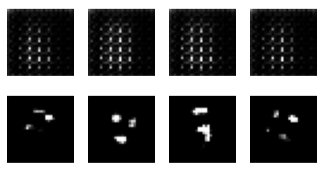
To see how well the generator is learning, we define a function that generates and displays images at different points during training. This function creates a batch of random noise, passes it through the generator to produce images, and uses Matplotlib to display them in a 4x4 grid. The pixel values are rescaled back from [-1, 1] to [0, 255] for proper visualization.

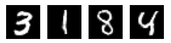
Finally, we start training the GAN using the train function we defined earlier. As the training progresses, the generated images should gradually become more realistic, allowing you to track the improvement of the generator over time.

# Function to generate and display images
def generate_and_save_images(model, epoch):
    # Generate random noise
    noise = tf.random.normal([16, NOISE_DIM])
    generated_images = model(noise, training=False)
    
    # Plot images in a 4x4 grid
    fig = plt.figure(figsize=(4, 4))
    for i in range(generated_images.shape[0]):
        plt.subplot(4, 4, i + 1)
        plt.imshow(generated_images[i, :, :, 0] * 127.5 + 127.5, cmap='gray')
        plt.axis('off')
    plt.show()

# Start training the GAN
train(train_dataset, EPOCHS)

Outputs :

Conclusion

Generative Adversarial Networks (GANs) represent a powerful and innovative approach to machine learning, capable of generating highly realistic data that mimics the real world. From creating stunning images and transforming them in various ways to enhancing the resolution of low-quality data, GANs have found applications across a diverse range of fields. While they come with challenges such as training instability and computational demands, their potential is vast and continually expanding. Whether you're a researcher, developer, or enthusiast, understanding and experimenting with GANs opens up exciting possibilities in artificial intelligence. As the technology evolves, GANs will likely play an increasingly crucial role in driving forward new advancements in AI and creative fields.

Experimenting with GANs allows you to understand how neural networks can create new data from scratch and opens the door to exciting possibilities in AI-driven creativity and research.