Deep Learning Fundamentals: How Neural Networks Learn

Deep learning is transforming industries, from healthcare and finance to entertainment and autonomous vehicles. As a subset of machine learning, it leverages complex neural networks to analyse vast amounts of data and make intelligent predictions. In this blog, we'll delve into the fundamentals of deep learning, exploring its core concepts, architectures, and applications to help you understand why it's such a game-changer in the world of artificial intelligence.

What Is Deep Learning?

Deep learning is a subfield of machine learning that focuses on training artificial neural networks with multiple layers, commonly known as deep neural networks. Unlike traditional machine learning approaches that depend heavily on manual feature engineering, deep learning models learn relevant features directly from raw data.

This learning happens through a hierarchical stack of layers, where each layer transforms its input into increasingly abstract representations. As data moves deeper into the network, simple patterns evolve into complex structures, allowing the model to capture intricate relationships. This ability makes deep learning highly effective for data-intensive and complex tasks such as image recognition, speech processing, natural language understanding, and game playing.

The rapid progress of deep learning is driven by three major factors: access to large-scale datasets, increased computational power, and the development of specialized architectures such as Convolutional Neural Networks and Recurrent Neural Networks. Together, these advances have made deep learning a central pillar of modern artificial intelligence.

Neural Networks: The Foundation of Deep Learning

Neural networks form the backbone of deep learning models. They consist of interconnected neurons organized into layers, where each connection carries a weight that is adjusted during training. By iteratively updating these weights to reduce prediction errors, neural networks learn meaningful patterns and representations from data.

This layered structure allows neural networks to model complex, non-linear relationships that are difficult to capture using traditional algorithms.

1. Layers and Architecture in Deep Neural Networks

A neural network is organized as a structured sequence of layers, each responsible for a specific stage of data transformation:

1. Input Layer - Serves as the entry point of the network by receiving raw features from the dataset. It passes this information forward without performing computations.

2. Hidden Layers - Perform the core learning process. Each hidden layer applies weighted sums followed by non-linear activation functions, enabling the network to extract progressively higher-level and more abstract features.

3. Output Layer - Produces the final prediction of the model, such as class probabilities for classification tasks or continuous values for regression problems.

The number of layers, the number of neurons per layer, and the overall architectural design determine the network’s expressive capacity. These choices directly influence how efficiently the model learns and how well it performs on unseen data.

2. Activation Functions and Non-Linear Modeling

Activation functions introduce non-linearity, allowing the network to capture complex relationships. After computing a weighted sum, each neuron applies an activation function such as ReLU, sigmoid, or tanh to generate its output.

Activation functions define how neurons transform input signals into outputs. Each function has distinct properties that make it suitable for specific layers and tasks in a neural network.

a. ReLU (Rectified Linear Unit)

ReLU outputs the input directly if it is positive and zero otherwise. It is computationally efficient and helps reduce the vanishing gradient problem, making it a default choice for hidden layers in deep networks. However, neurons can become inactive if they consistently receive negative inputs.

b. Leaky ReLU

Leaky ReLU is a variation of ReLU that allows a small, non-zero gradient for negative input values. This helps prevent neurons from becoming permanently inactive while retaining the efficiency of ReLU.

c. Sigmoid

The sigmoid function maps input values into a range between 0 and 1. It is commonly used in output layers for binary classification tasks, as its output can be interpreted as a probability. Sigmoid functions can suffer from vanishing gradients, making them less suitable for deep hidden layers.

d. Tanh (Hyperbolic Tangent)

Tanh maps inputs to a range between -1 and 1, producing outputs centered around zero. This property often leads to faster convergence than sigmoid in hidden layers. Like sigmoid, tanh can also experience vanishing gradient issues in deeper networks.

e. Softmax

Softmax converts a vector of values into a probability distribution where all outputs sum to one. It is widely used in the output layer of multi-class classification models to represent class probabilities.

f. Linear Activation

The linear activation function returns the input without modification. It is typically used in the output layer of regression models, where predictions are continuous values rather than class labels.

Each activation function influences how information flows through the network. Choosing the right activation function is essential for stable training, faster convergence, and accurate predictions.

3. Training and Optimization of Neural Networks

Training a neural network involves iteratively adjusting its weights to reduce the difference between predicted outputs and true targets. This process starts with a forward pass to generate predictions, followed by loss computation and gradient calculation using backpropagation.

Different optimization algorithms control how weights are updated during training, each with its own strengths:

a. Stochastic Gradient Descent (SGD)

SGD updates the network’s weights incrementally using gradients computed from individual samples or small batches. While it is simple and effective, it can converge slowly and may oscillate in regions of steep or uneven loss surfaces. Choosing the right learning rate is crucial for stable training.

b. SGD with Momentum

This variant of SGD adds a “momentum” term that accumulates past gradient updates, allowing the network to maintain movement in consistent directions and dampen oscillations. Momentum helps accelerate convergence, particularly when navigating narrow valleys in the loss landscape.

c. Adam (Adaptive Moment Estimation)

Adam combines the benefits of momentum and adaptive learning rates. It adjusts each parameter’s learning rate based on both the first moment (mean) and second moment (variance) of past gradients. This makes it highly effective for deep networks and complex tasks, often leading to faster and more stable convergence.

d. RMSprop

RMSprop divides the learning rate by a moving average of recent squared gradients. This normalization prevents updates from becoming too large or too small, which is especially helpful in recurrent neural networks and situations with non-stationary objectives.

e. Adagrad

Adagrad adapts learning rates individually for each parameter based on the accumulation of past squared gradients. It works well for sparse data, such as text or high-dimensional features, though its learning rate can decay too quickly over long training periods.

By selecting an appropriate optimizer, neural networks can train more efficiently, converge faster, and achieve better performance across different tasks and architectures.

4. Loss Functions for Model Learning

Loss functions are a critical component of neural networks, as they quantify how far the model’s predictions deviate from the actual target values. By providing this feedback, the loss function guides the optimization process, helping the network adjust its weights to improve accuracy over time.

Different tasks require different loss functions:

a. Mean Squared Error (MSE)

Widely used in regression tasks, MSE calculates the average squared difference between predicted and actual values. It penalizes larger errors more heavily, encouraging the model to make precise predictions.

b. Cross-Entropy Loss

Commonly used for classification tasks, cross-entropy measures the difference between predicted probability distributions and the true class labels. It encourages the model to assign higher probabilities to correct classes while reducing confidence in incorrect ones.

c. Other Loss Functions

Depending on the application, networks may use specialized loss functions such as Huber loss (for robust regression), Kullback-Leibler divergence (for probability distributions), or focal loss (for handling class imbalance in classification).

Choosing an appropriate loss function is essential, as it directly influences how the network learns and how well it generalizes to unseen data.

5. Overfitting and Regularization Techniques

Overfitting happens when a neural network learns the training data too well, capturing noise and minor fluctuations instead of underlying patterns. As a result, the model performs excellently on training data but poorly on unseen data, failing to generalize effectively.

To prevent overfitting, regularization techniques are applied during training:

a. Dropout

Randomly “drops” a fraction of neurons during each training iteration, forcing the network to learn redundant representations. This prevents reliance on any single neuron and improves generalization.

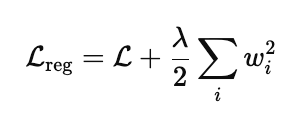
b. L2 Regularization (Weight Decay)

Adds a penalty to the loss function based on the squared magnitude of the weights. This discourages overly large weights, which can make the model overly sensitive to training data.

c. Other Techniques

Additional methods like early stopping (halting training when validation performance stops improving) and data augmentation (artificially expanding the training dataset) are also effective at reducing overfitting.

By incorporating these techniques, neural networks become more robust, maintaining strong performance on both training and unseen datasets.

6. Common Deep Learning Architectures

Deep learning's versatility and power stem from its diverse range of neural network architectures, each tailored to specific types of data and tasks. These architectures, ranging from simple feedforward networks to sophisticated models like transformers, have revolutionized various fields by enabling machines to understand and generate complex patterns. Understanding these common architectures is crucial, as they form the backbone of applications in image recognition, natural language processing, and more. In this section, we'll explore some of the most widely used deep learning architectures, highlighting their unique characteristics and use cases. Deep learning encompasses a variety of network architectures, each suited for different types of tasks:

1. Feedforward Neural Networks (FNNs): The simplest type of neural network, where data flows in one direction—from input to output—without cycles. FNNs are used for basic tasks such as image and text classification.

   
   

2. Convolutional Neural Networks (CNNs): Designed for processing grid-like data such as images. CNNs use convolutional layers to automatically and adaptively learn spatial hierarchies of features, making them highly effective for image recognition and computer vision tasks.

   
   

3. Recurrent Neural Networks (RNNs): Suitable for sequential data such as time series or natural language. RNNs have connections that form directed cycles, allowing them to maintain a state or memory of previous inputs. Variants like Long Short-Term Memory (LSTM) networks and Gated Recurrent Units (GRUs) address issues like vanishing gradients and are widely used in natural language processing (NLP).

   
   

4. Generative Adversarial Networks (GANs): Comprising two networks—a generator and a discriminator—that compete against each other. GANs are used for generating new data samples that resemble a given dataset, making them popular in tasks such as image generation and style transfer.

   
   

5. Transformers: A recent advancement in deep learning, transformers excel at handling sequential data and are the foundation of models like BERT and GPT. They use attention mechanisms to weigh the importance of different parts of the input data, enabling them to achieve state-of-the-art performance in NLP tasks.

Conclusion

Deep learning has reshaped the landscape of artificial intelligence by enabling machines to learn directly from data and solve problems that were once considered out of reach. Through layered neural networks, activation functions, optimization strategies, and carefully chosen loss functions, deep learning models can capture complex, non-linear patterns and make highly accurate predictions. Techniques such as regularization and advanced architectures further enhance their ability to generalize and perform reliably in real-world scenarios.

As explored in this blog, understanding the fundamentals—from neural network architecture to training dynamics and common deep learning models—provides a strong foundation for working with modern AI systems. As data continues to grow and computational resources advance, deep learning will remain a driving force behind innovation across industries, making it an essential area of knowledge for anyone interested in machine learning and artificial intelligence.

Whether you're just starting out or looking to deepen your knowledge, diving into the fundamentals of deep learning opens up exciting possibilities for exploring and creating the next generation of intelligent systems.