Weights And Biases with PyTorch to Track ML Experiments

Training a neural network is often described as “letting the model learn,” a phrase that can obscure the underlying process. In practice, learning is a well-defined optimization procedure that consists of repeatedly updating weights and biases to minimize a loss function. Every prediction produced by a neural network arises from how these parameters interact with the input data through a sequence of mathematical operations.

Understanding Weights and Biases with PyTorch is essential for building reliable machine learning systems. Knowing what they represent, how they evolve during training, and how they influence model behavior gives you real control over learning instead of blind trust in the framework. In this blog, we break down weights and biases in a neural network using PyTorch, explain how they drive learning, and show how to inspect and track them during experiments so training becomes transparent and debuggable rather than mysterious.

What Are Weights and Biases with PyTorch in a Neural Network?

Weights are the primary mechanism through which a neural network learns relationships in data. Each weight represents the importance of a specific input feature to a neuron’s output. When an input vector enters a layer, every input xix_ixi​ is multiplied by its corresponding weight wiw_iwi​. This multiplication determines how much that input contributes to the neuron’s overall signal.

Mathematically, the neuron computes a weighted sum:

z = w1 x1 + w2 x2 + ....+ wn xn

During training, weights are adjusted through backpropagation. The model compares its predictions to the true targets, computes an error, and then updates each weight in the direction that reduces that error. Over many iterations, useful features receive larger or more consistent weights, while irrelevant or noisy features are gradually dampened. This is how the network learns patterns instead of memorizing raw inputs.

In PyTorch, weights live inside layers as trainable parameters. For example, a nn.Linear layer internally maintains a weight matrix that is automatically registered as a parameter. PyTorch tracks these parameters, computes their gradients during backpropagation, and updates them using an optimizer. You usually do not manipulate weights directly, which is a blessing, because doing so by hand would be both tedious and error-prone.

import torch.nn as nn

layer = nn.Linear(3, 1)
print(layer.weight)

Output:
Parameter containing:
tensor([[-0.3372, -0.2815, -0.4091]], requires_grad=True)

Weights are stored as trainable parameters inside each layer. For example, nn.Linear(3, 1) creates a single neuron that expects three input features, represented by a weight tensor of shape (1, 3). Each value in this tensor corresponds to how strongly one input feature influences the neuron’s output. These weights are randomly initialized and marked with requires_grad=True, allowing PyTorch to track gradients and update them during backpropagation. As training progresses, these initially random values are adjusted to capture meaningful patterns in the data.

Biases are extra parameters added to a neuron that let it shift the activation function left or right. In practical terms, they act like an offset that allows a neuron to fire even when the input is zero or very small. Without a bias term, the neuron’s output depends entirely on the weighted sum of inputs, which means the activation function is always anchored at the origin. As a result, the model can only represent relationships that pass through (0, 0), which is an artificial and unnecessary constraint.

By including biases, a neural network gains the ability to model more realistic patterns. It can learn thresholds, offsets, and baseline behaviors, such as producing a non-zero output when all inputs are zero. This flexibility is crucial for approximating real-world functions, where important decision boundaries rarely align neatly with the origin. In short, biases give neurons the freedom to learn when to activate, not just how strongly to respond to inputs.

The full neuron equation becomes:

z = w1 x1 + w2 x2 + ....+ wn xn + b

Biases help models fit data more flexibly, especially when input features are zero or centered. In PyTorch:

print(layer.bias)

Output:
Parameter containing:
tensor([-0.2334], requires_grad=True)

Biases are trained alongside weights.

How Weights and Biases Learn During Training

Training a neural network is the process of systematically adjusting weights and biases so the model produces accurate predictions. In the forward pass, an input vector xxx is combined with the model parameters using a weighted sum and a bias term,

This linear combination represents the neuron’s raw signal, which is then passed through an activation function a = f ( z ) to introduce non-linearity. The network’s output y^​ is compared with the true target y using a loss function, which quantifies how far the prediction is from the desired result.

During backpropagation, the model computes gradients of the loss with respect to every weight and bias using the chain rule. These gradients indicate both the direction and magnitude by which each parameter influences the error,

In the parameter update step, an optimizer adjusts the parameters to reduce the loss, most commonly using gradient descent,

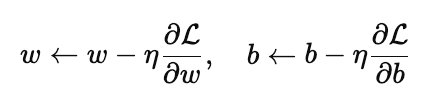
PyTorch handles gradient computation automatically.

loss.backward()
optimizer.step()

Each step slightly adjusts weights and biases in the direction that reduces error.

A Simple PyTorch Example

To see weights and biases in action, consider a small neural network built using PyTorch. This model takes two input features, passes them through a hidden layer with four neurons, applies a ReLU activation, and produces a single output.

import torch
import torch.nn as nn
import torch.optim as optim

model = nn.Sequential(
    nn.Linear(2, 4),
    nn.ReLU(),
    nn.Linear(4, 1)
)

criterion = nn.MSELoss()
optimizer = optim.SGD(model.parameters(), lr=0.01)

Each nn.Linear layer automatically creates a weight matrix and a bias vector. For nn.Linear(2, 4), the layer learns a weight matrix of shape (4, 2) and a bias vector of length 4. This means each of the four hidden neurons learns how to combine the two input features using its own set of weights and a bias. The final layer, nn.Linear(4, 1), combines the four hidden activations into a single output using another set of weights and a bias.

Before training begins, PyTorch initialises all weights and biases with small random values:

for name, param in model.named_parameters():
    print(name, param.data)

Output:
0.weight tensor([[ 0.1243, -0.6059],
        [ 0.4830,  0.5210],
        [-0.1174, -0.5163],
        [-0.6687, -0.5331]])
0.bias tensor([ 0.5467,  0.0030, -0.1447,  0.1606])
2.weight tensor([[-0.4484,  0.3220,  0.1569, -0.3476]])
2.bias tensor([-0.1226])

The printed output shows this clearly. The tensor 0.weight contains the weights for the first layer, where each row corresponds to one hidden neuron and each column corresponds to an input feature. The tensor 0.bias contains one bias value per hidden neuron. Similarly, 2.weight and 2.bias belong to the output layer, mapping the four hidden activations to a single prediction.

At this stage, these parameters do not represent anything meaningful. They are random starting points that allow the network to begin learning. During training, the loss function measures prediction error, backpropagation computes gradients for every weight and bias, and the optimizer updates them step by step. Over time, these initially random values are shaped into parameters that capture patterns in the data instead of guessing blindly.

Observing Weights and Biases During Training

Once training starts, weights and biases no longer sit still. They change slightly after every optimization step as the model tries to reduce prediction error. In this example, a small regression dataset with two input features is passed through the network for several epochs.

During each epoch, the model performs a forward pass to compute predictions, calculates the mean squared error loss, backpropagates gradients, and updates parameters using gradient descent:

import torch

# 10 samples, each with 2 features
inputs = torch.tensor([
    [1.0, 2.0],
    [2.0, 1.0],
    [3.0, 4.0],
    [4.0, 3.0],
    [5.0, 6.0],
    [6.0, 5.0],
    [7.0, 8.0],
    [8.0, 7.0],
    [9.0, 10.0],
    [10.0, 9.0]
])

# Corresponding targets (regression example)
targets = torch.tensor([
    [3.0],
    [3.0],
    [7.0],
    [7.0],
    [11.0],
    [11.0],
    [15.0],
    [15.0],
    [19.0],
    [19.0]
])

for epoch in range(5):
    optimizer.zero_grad()
    outputs = model(inputs)
    loss = criterion(outputs, targets)
    loss.backward()
    optimizer.step()

    print(f"Epoch {epoch}")
    for name, param in model.named_parameters():
        print(name, param.data.mean().item())

Outputs:
Epoch 0
0.weight -0.060705967247486115
0.bias 0.15582258999347687
2.weight 0.2464965283870697
2.bias 0.06442525237798691
Epoch 1
0.weight -0.37389811873435974
0.bias 0.11082422733306885
2.weight -0.11059954762458801
2.bias -0.047252438962459564
.
.
.

To make these changes visible, the mean value of each parameter tensor is printed after every epoch. The output shows that both weights and biases shift gradually across epochs. These shifts are not random. They reflect the optimizer adjusting parameters in response to the loss gradients.

Early in training, parameter values tend to change more noticeably as the model moves away from its random initialization. As training continues, updates usually become smaller, indicating that the model is approaching a set of weights and biases that better fit the data. Observing parameter values during training provides a practical way to confirm that learning is actually happening and that gradients are flowing correctly through the network.

Watching how weights and biases evolve during training is a practical way to catch common training pathologies early. Vanishing gradients show up when parameter values barely change across epochs, indicating that gradients are too small for effective learning and the network is essentially frozen. Exploding weights appear as rapidly growing parameter values, often jumping by large amounts between epochs, which can destabilize training and cause the loss to diverge. Dead neurons are revealed when certain weights or biases stop updating entirely, frequently in ReLU-based networks, meaning those neurons never activate and contribute nothing to the model. Monitoring parameter trends makes these issues visible instead of letting them silently sabotage training.

Why Initialization Matters

Weights and biases are not just placeholders the network figures out later. Their initial values directly influence how well and how fast a model learns. Poor initialization can lead to slow training, unstable updates, or complete failure to converge, even if the architecture and data are perfectly fine. In extreme cases, the network can get stuck before it learns anything meaningful.

At the start of training, weights determine the scale of activations and gradients flowing through the network. If weights are too large, activations and gradients can explode. If they are too small, gradients can vanish, leaving the model unable to update its parameters effectively. Biases also matter, as they control the initial activation behavior of neurons.

PyTorch uses sensible default initializations for most layers, designed to work well in common scenarios. However, explicit initialization is often useful, especially for deeper networks or when you want tighter control over training behavior. For example:

nn.init.xavier_uniform_(model[0].weight)
nn.init.zeros_(model[0].bias)
 
Output:
Parameter containing:
tensor([0., 0., 0., 0.], requires_grad=True)

Xavier initialization scales weights based on the number of input and output connections, helping keep activations stable across layers. Initializing biases to zero ensures neurons start without an artificial offset. As shown in the output, the bias tensor is explicitly set to zeros, making its starting behavior predictable.

Good initialization does not guarantee a perfect model, but it gives training a fair chance. With well-chosen initial weights and biases, learning tends to be faster, gradients behave more sensibly, and optimization becomes far more stable.

Conclusion

Understanding Weights and Biases with PyTorch removes much of the mystery around how neural networks actually learn. Every forward pass, loss calculation, and optimization step ultimately comes down to how weights scale input features and how biases shift neuron behavior. These parameters are not abstract concepts buried inside a framework. They are concrete values you can inspect, track, and reason about.

By working directly with weights and biases in PyTorch, you gain visibility into the learning process itself. Watching how parameters evolve during training helps diagnose issues like vanishing gradients, exploding weights, or inactive neurons long before they derail a model. Combined with sensible initialization strategies, this understanding leads to faster convergence and more stable training.

Once you are comfortable analyzing Weights and Biases with PyTorch, neural networks stop feeling like black boxes. They become systems you can debug, tune, and improve with confidence, which is exactly what separates trial-and-error modeling from disciplined machine learning practice.