Active Learning with PyTorch: Building a Smarter MNIST Classifier from Scratch

Active learning is all about teaching your machine learning model to ask the right questions. Instead of feeding it every piece of labeled data upfront, the model strategically selects the most informative samples for labeling thus saving time, effort, and cost.

In this hands-on guide, we’ll walk through building an active learning pipeline in PyTorch using the classic MNIST handwritten digits dataset. You’ll see how a model starts with a tiny labeled dataset, trains a simple CNN, identifies images it’s least confident about, and iteratively improves its accuracy by adding just the most valuable samples. By the end, you’ll have a working implementation, visualizations of the learning process, and a deeper understanding of how active learning can make your models smarter and more efficient.

Introduction to Active Learning

Active learning is a machine learning paradigm where the model is not a passive consumer of data but an active participant in the training process. Instead of labeling a large dataset all at once, active learning allows the model to selectively choose the most informative or uncertain samples to label. This approach is particularly valuable when labeling is expensive, time-consuming, or requires specialized expertise. By focusing only on the data that matters most, active learning can achieve high performance with far fewer labeled examples. Active learning has been successfully applied in a variety of domains, including:

1. Medical Imaging: Selecting the most uncertain scans for radiologist review to reduce labeling time while improving diagnostic models.

2. Natural Language Processing (NLP): Choosing ambiguous or rare text samples for annotation to enhance sentiment analysis, chatbot training, and entity recognition systems.

3. Speech Recognition: Actively querying unclear audio clips to improve transcription models in multiple languages.

4. Autonomous Vehicles: Prioritising edge cases from driving footage (e.g., unusual objects or weather conditions) for annotation to improve safety.

5. Industrial Inspection: Selecting uncertain defect images in manufacturing to refine visual quality control systems.

   
   

In essence, active learning bridges the gap between machine learning efficiency and human expertise. By allowing the model to ask for the data it truly needs, it reduces labelling overhead, speeds up development, and can lead to models that generalize better — all while using fewer labeled samples than traditional training methods.

Active Learning in Python with PyTorch for MNIST Handwritten Digit Classification

We’re now going to bring active learning to life by building a working example in Python with PyTorch, using the classic MNIST handwritten digits dataset. The idea is simple: start with just a small set of labeled images, train a convolutional neural network (CNN), and then let the model decide which new images it’s most unsure about. We’ll label those (simulated here) and feed them back into training. With each cycle, the model gets a little smarter without us having to label the entire dataset from the start. It’s a practical way to see how active learning saves effort while still boosting performance.

Step 1 – Importing Libraries and Setting Up the Environment

Before diving into the actual implementation, we need to bring in the tools that will make our active learning pipeline possible. PyTorch will handle the deep learning side of things, Torchvision gives us easy access to the MNIST dataset and helpful transformations, NumPy will take care of numerical operations, and Matplotlib will help us visualize our results. We’ll also import some utilities from torch.utils.data to manage labeled and unlabeled subsets during the active learning process.

import torch
import torch.nn as nn
import torch.optim as optim
import torch.nn.functional as F
from torchvision import datasets, transforms
from torch.utils.data import DataLoader, Subset, ConcatDataset
import numpy as np
import matplotlib.pyplot as plt

Step 2 – Defining the CNN Model

To classify handwritten digits, we’ll use a simple convolutional neural network (CNN). CNNs are well-suited for image tasks because they can automatically learn spatial patterns, such as strokes and curves, from pixel data. Our network has two convolutional layers to capture visual features, followed by fully connected layers that map these features to the 10 possible digit classes (0–9).

In the forward pass, the input image first goes through two convolutional layers with ReLU activation functions to detect patterns, followed by a max-pooling layer to reduce spatial dimensions while retaining key features. The result is flattened into a 1D vector, passed through a fully connected layer for further feature combination, and finally sent to the output layer, which produces class scores for each digit.

We’ll also set up our device configuration so the model can run on a GPU if one is available, falling back to the CPU otherwise.

# Simple CNN for MNIST
class SimpleCNN(nn.Module):
    def __init__(self):
        super().__init__()
        self.conv1 = nn.Conv2d(1, 32, 3, 1)
        self.conv2 = nn.Conv2d(32, 64, 3, 1)
        self.fc1 = nn.Linear(9216, 128)
        self.fc2 = nn.Linear(128, 10)

    def forward(self, x):
        x = F.relu(self.conv1(x))
        x = F.relu(self.conv2(x))
        x = F.max_pool2d(x, 2)
        x = torch.flatten(x, 1)
        x = F.relu(self.fc1(x))
        x = self.fc2(x)
        return x

# Setup device
device = torch.device("cuda" if torch.cuda.is_available() else "cpu")

Step 3 – Loading and Preparing the MNIST Dataset

The MNIST dataset is a collection of 70,000 grayscale images of handwritten digits (0–9), each sized at 28×28 pixels. It’s a classic benchmark for image classification tasks and is conveniently available through torchvision.datasets.

We’ll load both the training and test sets, applying a simple transformation to convert the images into tensors. For active learning, we’ll start with a small labeled set (1,000 images) and keep the rest as unlabeled data. During each cycle, we’ll acquire more data for labeling based on the model’s uncertainty.

To make the experiment reproducible, we’ll set a random seed, shuffle the indices, and split them into labeled and unlabeled pools right at the start.

# Load MNIST dataset (train + test)
transform = transforms.Compose([transforms.ToTensor()])
full_train = datasets.MNIST(root="./data", train=True, download=True, transform=transform)
test_dataset = datasets.MNIST(root="./data", train=False, download=True, transform=transform)

# Initial labeled set size and budget
initial_labeled_size = 1000
acquisition_size = 500
num_cycles = 5
batch_size = 64

# Create initial labeled and unlabeled indices
np.random.seed(42)
all_indices = np.arange(len(full_train))
np.random.shuffle(all_indices)

labeled_indices = list(all_indices[:initial_labeled_size])
unlabeled_indices = list(all_indices[initial_labeled_size:])

Step 4 – Defining the Training Function

To help our model learn from the labeled dataset, we’ll create a train function. This function takes the model, data loader, optimizer, and loss function (criterion) as inputs, and trains the model for one full pass (epoch) over the provided data.

During training, the model is set to training mode using model.train() so layers like dropout and batch normalization (if present) behave correctly. For each batch:

1. Data and labels are moved to the appropriate device (CPU or GPU).

2. The optimizer’s gradients are reset to avoid accumulation from previous steps.

3. The model generates predictions.

4. The loss between predictions and actual labels is calculated.

5. Backpropagation is performed to compute gradients.

6. The optimizer updates the model’s weights.

   
   

We also keep track of the total loss across all batches so we can monitor training performance.

def train(model, loader, optimizer, criterion):
    model.train()
    total_loss = 0
    for data, target in loader:
        data, target = data.to(device), target.to(device)
        optimizer.zero_grad()
        output = model(data)
        loss = criterion(output, target)
        loss.backward()
        optimizer.step()
        total_loss += loss.item()
    return total_loss / len(loader)

Step 5 – Defining the Testing Function

To measure how well our model is performing, we need a function to evaluate it on unseen data. The test function takes the model and a data loader as inputs, then returns the classification accuracy. Here’s what it does step-by-step:

1. Evaluation mode: The model is set to model.eval() so that layers like dropout and batch normalization behave in inference mode.

2. Disable gradient tracking: We wrap the loop in torch.no_grad() to save memory and computation since we’re not training.

3. Batch evaluation: For each batch, we move the data and labels to the correct device.

4. Prediction: The model outputs class scores, and we take the index of the highest score for each sample (argmax) as the predicted class.

5. Accuracy calculation: We compare predictions with the true labels and count the number of correct classifications.

6. Return accuracy: The total correct predictions are divided by the dataset size to give a value between 0 and 1.

def test(model, loader):
    model.eval()
    correct = 0
    with torch.no_grad():
        for data, target in loader:
            data, target = data.to(device), target.to(device)
            output = model(data)
            pred = output.argmax(dim=1)
            correct += pred.eq(target).sum().item()
    return correct / len(loader.dataset)

Step 6 – Calculating Uncertainty for Unlabeled Samples

The heart of active learning lies in deciding which samples the model should learn from next. Our get_uncertainty function measures how unsure the model is about each image in the unlabeled pool. We’ll use the Least Confidence strategy here, which works as follows:

1. Evaluation mode: Set the model to eval() to ensure consistent inference behavior.

2. Iterate over unlabeled data: Use a DataLoader to batch the unlabeled samples for efficient processing.

3. Prediction probabilities: Pass each batch through the model and apply a softmax to get class probabilities.

4. Find most confident class: For each sample, identify the maximum predicted probability.

5. Compute uncertainty: Subtract this value from 1. A high uncertainty means the model is less sure about its prediction.

6. Return scores: Convert the uncertainty scores into a NumPy array for further processing (like sorting and selecting top uncertain samples).

def get_uncertainty(model, dataset, indices):
    model.eval()
    uncertainties = []
    loader = DataLoader(Subset(dataset, indices), batch_size=batch_size)
    with torch.no_grad():
        for data, _ in loader:
            data = data.to(device)
            outputs = model(data)
            probs = F.softmax(outputs, dim=1)
            max_probs, _ = probs.max(dim=1)
            uncertainty = 1 - max_probs  # least confidence
            uncertainties.extend(uncertainty.cpu().numpy())
    return np.array(uncertainties)

Step 7 – Active Learning Loop

This step integrates all components to perform iterative model training, querying, and dataset expansion. In each cycle, the model is trained on the current labeled dataset, evaluated on the test dataset, and then used to select the most informative unlabeled samples based on uncertainty. These selected samples are then added to the labeled dataset, and the loop continues until all cycles are completed. Below are steps involved in each cycle:

1. Training: Load the labeled subset of the training data and train the model using the train() function.

2. Evaluation: Use the test() function to compute the model’s accuracy on the test dataset, providing feedback on performance improvements.

3. Uncertainty Calculation: Estimate the uncertainty of each unlabeled sample using get_uncertainty(). Higher uncertainty indicates samples the model is less confident about.

4. Query Selection: Select the top acquisition_size samples with the highest uncertainty for labeling.

5. Visualization: Display a few queried samples for inspection, showing both the image and its label.

6. Dataset Update: Add the newly labeled samples to the labeled dataset and remove them from the unlabeled pool.

   
   

This iterative process ensures that with each cycle, the model is exposed to the most valuable data points, steadily improving performance while minimizing labeling effort.

# Active Learning Loop
model = SimpleCNN().to(device)
criterion = nn.CrossEntropyLoss()
optimizer = optim.Adam(model.parameters())
test_loader = DataLoader(test_dataset, batch_size=batch_size)

test_accuracies = []
train_losses = []
labeled_sizes = []

for cycle in range(num_cycles):
    print(f"Cycle {cycle+1} / {num_cycles}")

    labeled_loader = DataLoader(Subset(full_train, labeled_indices), batch_size=batch_size, shuffle=True)

    train_loss = train(model, labeled_loader, optimizer, criterion)
    test_acc = test(model, test_loader)

    print(f"Train loss: {train_loss:.4f} | Test accuracy: {test_acc:.4f}")

    test_accuracies.append(test_acc)
    train_losses.append(train_loss)
    labeled_sizes.append(len(labeled_indices))

    if cycle == num_cycles - 1:
        break

    uncertainties = get_uncertainty(model, full_train, unlabeled_indices)
    query_indices = np.argsort(uncertainties)[-acquisition_size:]
    new_indices = [unlabeled_indices[i] for i in query_indices]

    # Show some queried samples
    print(f"Queried sample indices: {new_indices[:5]} (showing first 5)")

    # Visualize queried samples at this cycle
    fig, axs = plt.subplots(1, 5, figsize=(12, 3))
    for i, idx in enumerate(new_indices[:5]):
        img, label = full_train[idx]
        axs[i].imshow(img.squeeze(), cmap='gray')
        axs[i].set_title(f"Label: {label}")
        axs[i].axis('off')
    plt.suptitle(f"Cycle {cycle+1} - Queried Samples")
    plt.show()

    labeled_indices.extend(new_indices)
    unlabeled_indices = [idx for idx in unlabeled_indices if idx not in new_indices]

print("Active learning finished.")

Output:

Step 8 – Visualizing Active Learning Progress

To track how the model evolves across cycles, we plot three key metrics side by side: test accuracy versus cycle to show how performance improves as more informative samples are added; train loss versus cycle to reveal how prediction errors decrease as the model learns; and labeled set size versus cycle to capture how the training dataset grows with each iteration. Together, these plots provide a clear visual narrative of the active learning journey, making it easy to assess how effectively the strategy improves the model over time.

plt.figure(figsize=(12, 4))

# Plot Test Accuracy vs Cycle
plt.subplot(1, 3, 1)
plt.plot(range(1, num_cycles + 1), test_accuracies, marker='o')
plt.title('Test Accuracy vs Cycle')
plt.xlabel('Active Learning Cycle')
plt.ylabel('Accuracy')

# Plot Train Loss vs Cycle
plt.subplot(1, 3, 2)
plt.plot(range(1, num_cycles + 1), train_losses, marker='o', color='orange')
plt.title('Train Loss vs Cycle')
plt.xlabel('Active Learning Cycle')
plt.ylabel('Loss')

# Plot Labeled Set Size vs Cycle
plt.subplot(1, 3, 3)
plt.plot(range(1, num_cycles + 1), labeled_sizes, marker='o', color='green')
plt.title('Labeled Set Size vs Cycle')
plt.xlabel('Active Learning Cycle')
plt.ylabel('Number of Samples')

plt.tight_layout()
plt.show()

Output:

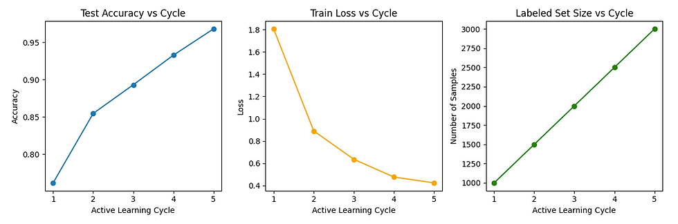
Through this step-by-step active learning process, we have demonstrated how a model can start with minimal labeled data, strategically select the most informative samples, and progressively improve its performance over multiple cycles. From computing uncertainties and querying new data points to retraining the model and visualizing results, each cycle builds upon the last, ensuring that labeling efforts yield maximum impact. This approach not only reduces labeling costs but also accelerates the path to a high-performing model without needing exhaustive data annotation from the outset.

Conclusion

Active learning stands out as a powerful paradigm for optimizing machine learning workflows when labeled data is scarce or expensive to obtain. By intelligently selecting the most informative data points for labeling, it focuses human annotation efforts on areas where the model is most uncertain, leading to steeper and more efficient learning curves. This approach is especially valuable in domains like image classification, NLP, medical diagnostics, and autonomous systems, where the cost of labeling can be prohibitively high. Beyond reducing annotation expenses, active learning also accelerates model improvement by continuously refining decision boundaries with the most impactful examples. As AI projects grow in scale and complexity, integrating active learning into the development pipeline can transform an overburdened, resource-heavy labeling process into a streamlined, cost-effective system that delivers high-performance models with fewer labeled samples. Ultimately, its strategic use bridges the gap between limited labeled data and the demand for robust AI systems, making it an essential tool in the modern machine learning toolkit.