

What is Q-Learning? Concepts, Formula, and Example
- 17 hours ago
- 6 min read
Q-learning continues to sit at the heart of Reinforcement Learning, powering systems that learn directly from interaction instead of relying on predefined rules. From game-playing agents to robotics and decision-making systems, it remains one of the most practical and widely used algorithms for teaching machines how to act in uncertain environments. Despite the rise of deep reinforcement learning and neural approaches, Q-learning still holds its ground as a foundational method—simple in idea, yet powerful enough to demonstrate how intelligent behavior can emerge from trial, error, and reward-driven learning.
In this blog, we’ll break down what Q-learning is within the broader context of Reinforcement Learning, starting with its core concepts and connection to Markov Decision Processes. We’ll walk through the Q-function, the Bellman equation, and how the learning process actually unfolds step by step. You’ll also explore real-world applications, key advantages and limitations, and finally see how Q-learning translates into practice, with a reference to a hands-on implementation to tie everything together.

What is Q-Learning and Why It Matters in RL
Q-learning is a model-free reinforcement learning algorithm that teaches an agent how to make optimal decisions by interacting with an environment. Instead of relying on a predefined model of how the environment works, it learns purely from experience. The core idea is simple: for every state–action pair, the agent estimates a value called the Q-value, which represents the expected future reward of taking that action in that state. Over time, by exploring different actions and receiving rewards or penalties, the agent updates these Q-values and gradually learns which actions lead to the best outcomes.
What makes Q-learning important in reinforcement learning is its ability to learn an optimal policy without needing a model of the environment. It works directly within the framework of Markov Decision Processes, using the Bellman equation to iteratively improve its estimates until it converges to the best possible strategy. This makes it highly practical for real-world problems where the environment is unknown or too complex to model. From game-playing agents to robotics and decision systems, Q-learning acts as a foundational algorithm that demonstrates how intelligent behavior can emerge from simple reward-driven learning.
Model-Free Learning and Optimal Policy in Q-Learning
One of the most powerful aspects of Q-learning is its model-free nature. In reinforcement learning, a model typically means knowing two things in advance .i.e. the transition dynamics (how the environment moves from one state to another) and
the reward function (what reward you get after each action).
Most real-world problems don’t hand you this information neatly packaged. The environment is messy, unpredictable, or simply unknown. Q-learning sidesteps this entirely.
Instead of trying to understand how the environment works, it focuses on what works best through direct interaction. The agent takes an action, observes the outcome, receives a reward, and updates its knowledge. No assumptions, no prior map, just experience.
This is why Q-learning is called off-policy. It doesn’t need to follow the optimal strategy while learning it. The agent can explore randomly and still learn the optimal policy in the background. A common way to handle this exploration is through the epsilon-greedy strategy. In an epsilon-greedy approach, the agent follows a simple rule:
With probability ε (epsilon), it chooses a random action (exploration)
With probability 1 − ε, it chooses the action with the highest Q-value (exploitation)
This balance between exploration and exploitation is critical. If the agent only exploits, it may get stuck with suboptimal decisions because it never tries anything new. If it only explores, it never settles on a good strategy. Epsilon-greedy gives a controlled way to do both.
What makes this especially important in Q-learning is that the learning process is independent of the behavior used to collect data. Even while the agent is taking random actions during exploration, it is still updating its Q-values toward the optimal policy using the best possible future reward estimates. In other words, it can behave imperfectly while still learning the perfect strategy.
This separation between learning and acting is what allows Q-learning to thrive in uncertain environments. The agent doesn’t need a perfect plan upfront. It experiments, adjusts, and gradually improves, until what started as random behavior turns into consistently optimal decisions.
Q-Learning Within The Markov Decision Process
Even though Q-learning is model-free, it doesn’t exist in chaos. It operates within the structured framework of a Markov Decision Process (MDP), which provides the mathematical backbone for most reinforcement learning problems. An MDP defines how an agent interacts with its environment and is typically described using four key components:
States (S): All possible situations the agent can be in
Actions (A): The set of choices available to the agent in each state
Reward Function (R): Feedback received after taking an action
Transition Dynamics (P): The probability of moving from one state to another after an action
At the heart of this framework lies the Markov property, which states that:
The future state depends only on the current state and action, not on the sequence of events that came before.
This assumption is what makes learning tractable. It allows the agent to treat each state as a complete and self-contained representation of the environment at that moment.
Q-learning heavily relies on this property. When the agent updates its Q-values, it assumes that the current state holds all the relevant information needed to evaluate the next action. It doesn’t try to remember long histories or track past trajectories. Instead, it focuses only on the present state and the immediate transition that follows.
Without the Markov property, this approach would break down. If hidden or past information influenced future outcomes, the agent’s updates would become unreliable. The same state-action pair could lead to different results depending on unseen history, making it impossible for Q-learning to converge to consistent values.
So while Q-learning ignores the need to explicitly model transition probabilities or reward distributions, it still depends critically on the structure of the MDP. The framework ensures that the learning process remains stable, consistent, and mathematically grounded. In a way, the MDP provides the rules of the game, while Q-learning figures out how to win it through experience.
The Role of the Bellman Equation in Learning
At the core of Q-learning lies the idea of iterative improvement, driven by the Bellman optimality principle. Instead of computing the optimal policy in a single step (which would require complete knowledge of the environment’s dynamics), Q-learning refines its estimates gradually through repeated interaction. This is what makes it both practical and powerful in unknown environments.
The Bellman principle essentially states that:
The value of a decision now depends on the immediate reward plus the value of the best possible decisions in the future.
In the context of Q-learning, this idea is translated into an update rule that continuously improves the estimate of the action-value function.
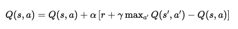
This equation formalizes how learning happens at every step. Let’s break it down more mathematically and intuitively:
1. Current Estimate:
The agent maintains a value Q(s,a), which represents the expected cumulative reward of taking action a in state s and following the optimal strategy thereafter.
2. Observed Transition:
After taking action a, the agent receives an immediate reward r and transitions to a new state s′.
3. Bootstrapped Target (Bellman Target):
Instead of waiting to observe long-term outcomes, Q-learning uses a bootstrapping approach. It estimates the future reward using:

where:
γ∈[0,1] is the discount factor, controlling how much future rewards matter
maxa′Q(s′,a′)\max_{a'} Q(s',a')maxa′Q(s′,a′) represents the best possible future value from the next state
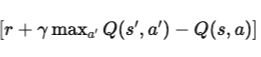
4. Temporal Difference (TD) Error:
The difference between the new estimate and the old estimate, this error measures how “wrong” the current estimate was.:
5. Update Step:
The Q-value is adjusted in the direction of this error:
Q(s,a) ← Q(s,a) + α⋅δ
where α is the learning rate, controlling how aggressively the agent updates its beliefs.
Over time, as the agent explores the environment and updates its Q-values repeatedly, these estimates begin to stabilize. Under certain conditions like sufficient exploration and a properly tuned learning rate Q-learning is mathematically guaranteed to converge to the optimal action-value function.
Once the optimal Q-values are learned, deriving the optimal policy becomes trivial:
For any given state, simply choose the action with the highest Q-value
No explicit policy was ever stored or optimized directly. It emerges naturally from the learned values.


