Implementing Neural Networks for Image Classification on the CIFAR-10 Dataset Using TensorFlow in Python

Ever wondered how modern devices distinguish between a picture of a pet and a vehicle? This capability is powered by image classification, one of the most important and practical applications of deep learning. Image classification allows machines to analyze visual data and automatically assign labels to images based on their content.

To accomplish this task, we use neural networks, a core deep learning algorithm designed to learn patterns and features from images. By analyzing thousands of labeled examples, a neural network gradually learns to recognize shapes, textures, and colors that help it differentiate between categories. One of the most popular datasets used to explore this concept is the CIFAR-10 dataset, which provides a diverse collection of images representing everyday objects.

In this guide, we will explore how image classification works by implementing a neural network on the CIFAR-10 dataset using TensorFlow in Python. Through this process, we will gain practical insight into how neural networks process visual data, learn from training examples, and make predictions on unseen images. This hands-on experience builds a strong foundation for more advanced projects in computer vision and deep learning.

What is CIFAR-10 Dataset in TensorFlow (Python)?

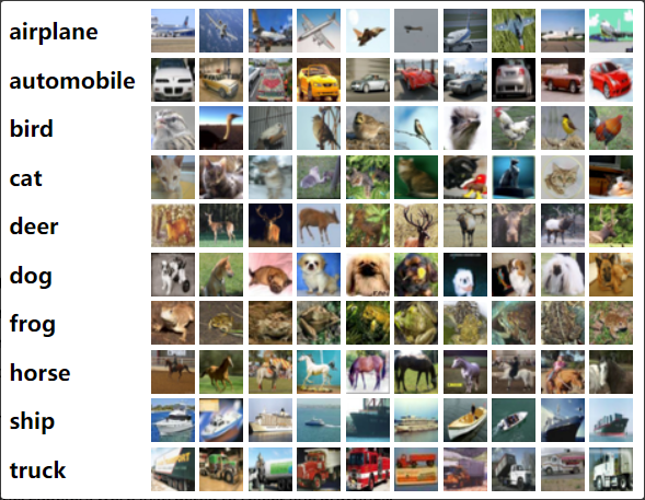
The CIFAR-10 dataset is a standard benchmark in computer vision and deep learning, consisting of 60,000 color images of size 32x32 pixels. These images are divided into 10 categories, such as airplanes, cars, birds, cats, dogs, and trucks. Each image is labeled, making CIFAR-10 a classic multiclass classification problem. The dataset is split into 50,000 training images and 10,000 test images, allowing us to train neural networks and evaluate how well they generalize to new, unseen data.

Using CIFAR-10 in TensorFlow (Python) is convenient because TensorFlow provides built-in functions to load and preprocess the dataset, enabling us to focus on building and training models without worrying about data preparation. The dataset is widely supported in tutorials, research papers, and educational resources, which makes it an ideal starting point for anyone learning image classification.

The importance of CIFAR-10 lies in its balance of simplicity and challenge. The images are small, so experiments can run quickly on standard hardware, yet they are complex enough to require neural networks to learn meaningful features, such as shapes, textures, and colors. By working with CIFAR-10, we gain practical experience in designing, training, and evaluating neural network models, which can then be applied to more advanced datasets and real-world applications like autonomous vehicles, object detection, and AI-powered visual recognition systems.

In short, CIFAR-10 provides a practical, hands-on platform for understanding deep learning, mastering image classification, and learning how neural networks extract and use visual features to make accurate predictions.

Implementation: Building the CIFAR-10 Classifier

Now that we understand the CIFAR-10 dataset and the concepts behind image classification and neural networks, we can move on to the practical part of this guide. In this section, we will implement an image classification model using the CIFAR-10 dataset with TensorFlow in Python.

Using TensorFlow’s Keras API, we will build and train a neural network capable of learning visual patterns from the dataset and predicting the correct class for new images. The implementation will demonstrate how deep learning models can process image data and gradually learn meaningful features that allow them to distinguish between different object categories.

In the following steps, we will walk through the process of preparing the dataset, constructing the neural network, training the model, and evaluating its performance on unseen images. This hands-on implementation will provide practical insight into how neural networks are applied to real-world image classification tasks.

Step 1: Setting Up Your Environment

Before building a neural network for image classification, you need to install TensorFlow and a few supporting libraries. TensorFlow provides the deep learning framework, while NumPy helps with numerical operations and Matplotlib is used to visualize images from the dataset.

You can install the required libraries using pip:

pip install tensorflow numpy matplotlib

Once the installation is complete, your Python environment will be ready for implementing the CIFAR-10 image classification model using TensorFlow.

Step 2: Loading, Preprocessing, and Visualizing the CIFAR-10 Dataset

TensorFlow provides built-in utilities that make it easy to load the CIFAR-10 dataset directly within Python. The dataset contains 60,000 small color images categorized into 10 different object classes such as airplanes, cars, cats, and trucks.

After loading the dataset, the pixel values are normalized so they fall between 0 and 1. Normalization improves neural network training because it keeps input values within a consistent range.

The following code loads the dataset, normalizes the images, defines class labels, and visualizes sample images from the training data.

import tensorflow as tf
import numpy as np
import matplotlib.pyplot as plt
from tensorflow.keras.datasets import cifar10

# Load the CIFAR-10 dataset
(train_images, train_labels), (test_images, test_labels) = cifar10.load_data()

# Normalize pixel values to be between 0 and 1
train_images, test_images = train_images / 255.0, test_images / 255.0

# Define class names
class_names = ['airplane', 'automobile', 'bird', 'cat', 'deer',
               'dog', 'frog', 'horse', 'ship', 'truck']

# Plot some images from the dataset
def plot_images(images, labels, class_names):
    plt.figure(figsize=(15, 15))
    for i in range(25):
        plt.subplot(5, 5, i + 1)
        plt.imshow(images[i])
        plt.title(class_names[labels[i][0]])
        plt.axis('off')
    plt.show()
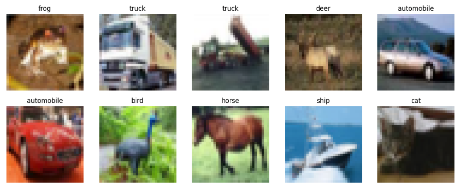
plot_images(train_images, train_labels, class_names)

Visualizing the dataset helps confirm that the images and labels were loaded correctly. It also gives a quick overview of the different object categories that the neural network will learn to classify.

Step 3: Building the Convolutional Neural Network (CNN)

To classify images in the CIFAR-10 dataset, we build a Convolutional Neural Network (CNN) using TensorFlow’s Keras API. CNNs are specifically designed for image data because they can automatically learn spatial features such as edges, textures, and object shapes.

The model architecture below contains several key components. Convolutional layers extract important visual features from the images, while max-pooling layers reduce spatial dimensions and help the model focus on the most relevant patterns. After feature extraction, dense layers perform the final classification into one of the ten CIFAR-10 categories.

The following code defines and compiles a simple CNN model.

from tensorflow.keras import layers, models

# Build the CNN model
model = models.Sequential([
    layers.Conv2D(32, (3, 3), activation='relu', input_shape=(32, 32, 3)),
    layers.MaxPooling2D((2, 2)),
        layers.Conv2D(64, (3, 3), activation='relu'),
    layers.MaxPooling2D((2, 2)),
        layers.Conv2D(64, (3, 3), activation='relu'),
        layers.Flatten(),
    layers.Dense(64, activation='relu'),
    layers.Dense(10, activation='softmax')])

# Compile the model
model.compile(
    optimizer='adam',
    loss='sparse_categorical_crossentropy',
    metrics=['accuracy'])

# Display model architecture
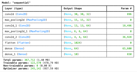
model.summary()

This CNN architecture gradually learns visual features from the CIFAR-10 images and then uses fully connected layers to classify them into the correct object category. The Adam optimizer is used to update model weights efficiently, while sparse categorical crossentropy measures how well the model predicts the correct class.

Displaying the model summary provides an overview of each layer in the network, including output shapes and the number of trainable parameters.

Step 4: Training the Model

After building and compiling the convolutional neural network, the next step is to train the model using the CIFAR-10 training dataset. During training, the neural network learns to recognize patterns in the images by adjusting its internal weights based on prediction errors.

TensorFlow provides the fit() function to train the model for multiple epochs. An epoch represents one complete pass through the entire training dataset. With each epoch, the model attempts to minimize the loss function and improve its classification accuracy. At the same time, the model is evaluated on the validation dataset so we can observe how well it performs on unseen data.

The following code trains the CNN model for ten epochs using the training images and labels, while validating the model using the test dataset.

# Model Training
history = model.fit(
    train_images,
    train_labels,
    epochs=10,
    validation_data=(test_images, test_labels))

When this code is executed, TensorFlow displays the training progress for each epoch. The output shows metrics such as accuracy, loss, validation accuracy, and validation loss, which help monitor how the model improves during training.

Epoch 1/101563/1563 ━━━━━━━━━━━━━━━━━━━━ 79s 49ms/step - accuracy: 0.3444 - loss: 1.7613 - val_accuracy: 0.5215 - val_loss: 1.3080
...
Epoch 10/101563/1563 ━━━━━━━━━━━━━━━━━━━━ 80s 48ms/step - accuracy: 0.7807 - loss: 0.6208 - val_accuracy: 0.7075 - val_loss: 0.8749

As training progresses, the model’s accuracy increases while the loss decreases. This indicates that the neural network is gradually learning meaningful visual patterns from the CIFAR-10 images and improving its classification performance.

Step 5: Evaluating the Model

After training the neural network, the next step is to evaluate its performance on the test dataset. This helps determine how well the model generalizes to new images that were not part of the training data.

TensorFlow provides the evaluate() function, which calculates the model’s loss and accuracy using the test dataset. These metrics provide a clear indication of how effectively the trained CNN can classify images from the CIFAR-10 dataset.

The following code evaluates the model:

# Model Evaluation
test_loss, test_acc = model.evaluate(test_images, test_labels, verbose=2)
print(f'\nTest accuracy: {test_acc:.4f}')

After running the evaluation, TensorFlow outputs the performance metrics for the test dataset.

313/313 - 5s - 16ms/step - accuracy: 0.7075 - loss: 0.8749
Test accuracy: 0.7075

The results show that the trained convolutional neural network achieves a test accuracy of approximately 70.75%, indicating that the model can correctly classify most images in the CIFAR-10 test dataset.

Step 6: Visualizing Training Progress

Visualizing training results helps better understand how the neural network learned during the training process. By plotting training and validation accuracy across epochs, it becomes easier to observe trends such as improvements in performance or potential overfitting.

The history object returned during model training stores the accuracy and validation accuracy values for each epoch. These values can be used to generate a simple accuracy graph.

import matplotlib.pyplot as plt

# Plot training & validation accuracy valuesplt.plot(history.history['accuracy'])
plt.plot(history.history['val_accuracy'])
plt.title('Model Accuracy')
plt.xlabel('Epoch')
plt.ylabel('Accuracy')
plt.legend(['Train', 'Validation'], loc='upper left')
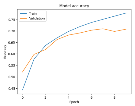
plt.show()

This visualization displays how the model’s accuracy improves during training while also showing how well it performs on validation data. Comparing these two curves helps determine whether the model is learning effectively or beginning to overfit the training dataset.

In addition to accuracy, it is also useful to visualize the loss values during training. Loss measures how far the model’s predictions are from the actual labels, so observing the training and validation loss across epochs helps determine whether the model is learning effectively.

By plotting both training loss and validation loss, it becomes easier to identify issues such as underfitting or overfitting. Ideally, the loss should decrease steadily as the model learns from the dataset.

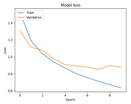
The following code generates a graph showing how the loss changes throughout the training process.

# Plot training & validation loss values
plt.plot(history.history['loss'])
plt.plot(history.history['val_loss'])
plt.title('Model Loss')
plt.xlabel('Epoch')
plt.ylabel('Loss')
plt.legend(['Train', 'Validation'], loc='upper left')
plt.show()

This plot shows how the model’s error changes during each training epoch. As training progresses, the loss should generally decrease, indicating that the neural network is improving its predictions.

Conclusion

Implementing a neural network on the CIFAR-10 dataset using TensorFlow provides a practical introduction to image classification with deep learning. By working through the process of loading and preprocessing the dataset, building a convolutional neural network, training the model, and evaluating its performance, we gain a clear understanding of how modern computer vision systems are developed.

Using TensorFlow’s Keras API simplifies the process of creating and training neural networks while still providing powerful tools for experimentation and optimization. The results from training and evaluation demonstrate how CNNs can learn meaningful visual patterns and classify images into multiple categories with reasonable accuracy.

Visualizing training metrics such as accuracy and loss also helps interpret the model’s learning behavior and identify potential improvements. This hands-on implementation forms a strong starting point for experimenting with deeper architectures, hyperparameter tuning, and more advanced deep learning techniques used in real-world computer vision applications.