Implementing k-Nearest Neighbors (kNN) on the Iris Dataset in Python

The k-Nearest Neighbors (kNN) algorithm is a simple yet powerful machine learning technique used for both classification and regression tasks. Its ease of use and effectiveness make it a popular choice for beginners and experienced practitioners alike.

In this blog, we will explore how to implement kNN using Python's scikit-learn library, focusing on the classic Iris dataset, a staple in the machine learning community.

k-Nearest Neighbors (kNN) in Python

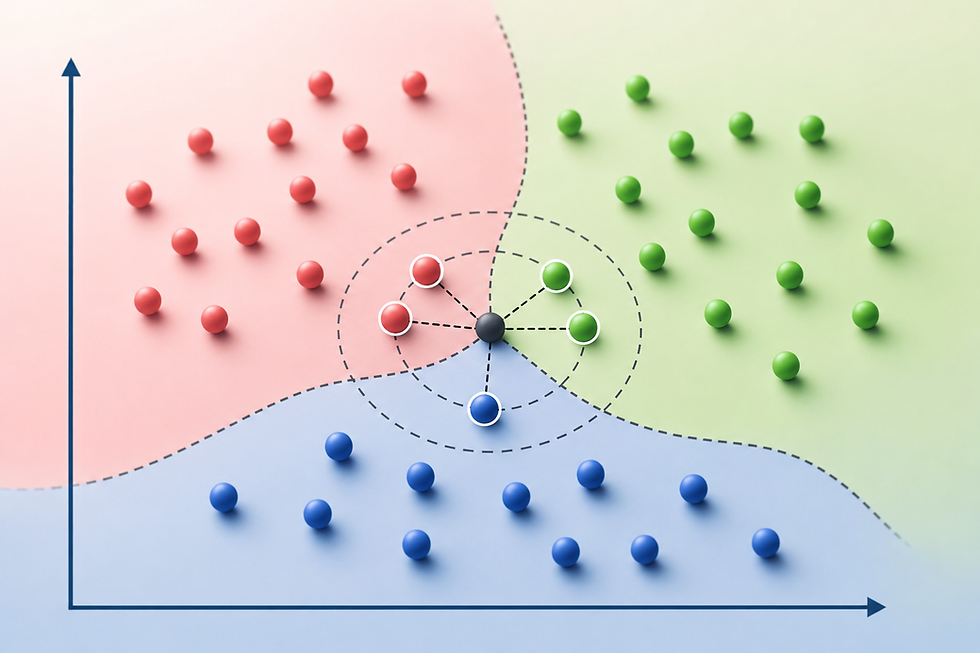
k-Nearest Neighbors (kNN) is a simple yet powerful algorithm used for both classification and regression tasks in machine learning. In Python, kNN can be easily implemented using the KNeighborsClassifier and KNeighborsRegressor classes from the scikit-learn library. The kNN algorithm works by finding the 'k' most similar instances in the training data to a given input sample and then predicting the output based on these neighbors. For classification, the predicted class is determined by a majority vote among the 'k' nearest neighbors, while for regression, the output is typically the average of the neighbors' values.

The similarity between instances is commonly measured using distance metrics such as Euclidean distance, Manhattan distance, or Minkowski distance, with Euclidean distance being the most popular choice. The selection of 'k' is crucial, as a smaller 'k' can lead to a model sensitive to noise, while a larger 'k' may result in a model that overlooks important patterns. One of the key strengths of kNN is its simplicity and ease of implementation, requiring minimal assumptions about the underlying data distribution. Additionally, kNN is a non-parametric algorithm, meaning it does not assume a specific form for the mapping function from input to output, making it highly flexible. However, kNN can be computationally expensive, especially with large datasets, as it requires storing all the training data and calculating distances for each prediction.

To optimize performance, techniques such as KD-Trees or Ball Trees are often used for efficient nearest neighbor searches. Despite these challenges, kNN remains a widely used and intuitive method, particularly useful as a baseline model and in situations where model interpretability and simplicity are valued.

The Iris Dataset in Python

The Iris dataset is one of the most well-known and commonly used datasets in the field of machine learning and data science. It serves as a standard benchmark for testing and comparing various machine learning algorithms. The dataset consists of 150 samples of iris flowers, with each sample having four features and a corresponding class label. The features represent the physical dimensions of the flowers and include:

1. Sepal length (in centimeters)

2. Sepal width (in centimeters)

3. Petal length (in centimeters)

4. Petal width (in centimeters)

Each flower in the dataset belongs to one of three species:

1. Iris setosa

2. Iris versicolor

3. Iris virginica

The class labels are encoded as integers, with 0 representing Iris setosa, 1 representing Iris versicolor, and 2 representing Iris virginica.

The Iris dataset is often used for classification tasks, where the goal is to predict the species of an iris flower based on its features. The dataset is particularly valuable for its simplicity and balance, as it contains an equal number of samples (50) for each species. Moreover, the four features exhibit enough variation to make the classification task non-trivial, while still being manageable for visual exploration and understanding.

The dataset can be easily loaded in Python using the scikit-learn library, which provides it as a built-in dataset. The balanced and well-documented nature of the Iris dataset makes it an excellent choice for demonstrating machine learning techniques, including decision trees, support vector machines, k-nearest neighbors, and more. It also serves as a foundational dataset for educational purposes, helping newcomers to the field understand fundamental concepts in machine learning and data analysis.

Implementing k-Nearest Neighbors (kNN) in Python

Implementing k-Nearest Neighbors (kNN) in Python is straightforward and efficient, thanks to the robust functionalities provided by the scikit-learn library. The process begins by importing the necessary classes, such as KNeighborsClassifier or KNeighborsRegressor, depending on whether the task is classification or regression. The dataset, typically loaded from a library like scikit-learn or imported from a CSV file, is then split into training and testing sets. The model is initialized by specifying the number of neighbors 'k' and the distance metric, with Euclidean distance being the default.

The training process involves simply storing the training data, as kNN is a lazy learning algorithm that does not create a model until a prediction is required. When making predictions, the algorithm calculates the distances between the input sample and all training samples, selects the 'k' closest ones, and determines the output based on these neighbors—either by majority vote for classification or averaging for regression. Performance evaluation is conducted using metrics like accuracy for classification or mean squared error for regression, providing insights into the model's effectiveness.

The implementation also allows for fine-tuning of parameters such as 'k' and distance metric to optimize model performance. Overall, implementing kNN in Python is a user-friendly process that balances simplicity and flexibility, making it a popular choice for both beginners and experienced practitioners in machine learning. Let's walk through the implementation of kNN on the Iris dataset using scikit-learn.

Step 1: Import Libraries

To build the k-Nearest Neighbors (kNN) classifier, the required libraries are first imported from scikit-learn. These libraries provide utilities for loading the Iris dataset, splitting the data into training and testing sets, building the kNN model, and evaluating prediction accuracy.

from sklearn.datasets import load_iris
from sklearn.model_selection import train_test_split
from sklearn.neighbors import KNeighborsClassifier
from sklearn.metrics import accuracy_score

Step 2: Load the Dataset

The Iris dataset is loaded using load_iris() and separated into input features (X) and target labels (y). The dataset contains measurements of iris flowers, such as petal and sepal dimensions, which are used to classify different flower species.

# Load the Iris dataset
iris = load_iris()
X = iris.data # Features
y = iris.target # Target labels

Step 3: Split the Data

The dataset is divided into training and testing subsets using train_test_split(). The training data is used to teach the kNN model patterns within the dataset, while the testing data helps evaluate how well the model performs on unseen samples. Setting random_state=42 ensures reproducible results across executions.

# Split the dataset into training and testing sets
X_train, X_test, y_train, y_test = train_test_split(X, y, test_size=0.3, random_state=42)

Step 4: Create and Train the kNN Model

A KNeighborsClassifier is created with k=3, meaning the model will classify new samples based on the three nearest neighboring data points. The model is then trained using the training dataset with the fit() function. During this process, the classifier stores the training data and learns the structure needed for future predictions.

# Create a kNN Classifier with k=3
knn = KNeighborsClassifier(n_neighbors=3)

# Train the model
knn.fit(X_train, y_train)

Step 5: Make Predictions

After training, the kNN classifier predicts the classes of the testing samples using the predict() function. The model determines the nearest neighbors for each test sample and assigns the most common class among them as the prediction.

# Make predictions on the test set
y_pred = knn.predict(X_test)

Step 6: Evaluate the Model

The model’s performance is evaluated using accuracy_score(), which measures the percentage of correctly classified samples in the testing dataset. The resulting accuracy value provides a simple indication of how effectively the kNN classifier can distinguish between different iris flower species based on their feature values.

# Calculate accuracy
accuracy = accuracy_score(y_test, y_pred)
print(f"Accuracy: {accuracy:.2f}")

In this example, we've chosen k=3 neighbors. The choice of 'k' can significantly impact the model's performance, and it's often selected through cross-validation.

Choosing the Right 'k'

Selecting the optimal value of 'k' is crucial for the performance of the kNN algorithm. A smaller 'k' value can lead to overfitting, as the model might be too sensitive to noise in the data. On the other hand, a larger 'k' value can result in underfitting, as the model might oversimplify the decision boundary.

To find the best 'k', you can use techniques like cross-validation, where the data is split into multiple training and testing sets to evaluate the model's performance for different 'k' values. The 'k' that results in the highest average accuracy across these splits is typically chosen.

Step 7: Visualizing the kNN Decision Boundary

To better understand how the kNN classifier separates different classes, a decision boundary visualization is created using Matplotlib. The code first defines the plotting boundaries based on the feature ranges and generates a mesh grid of points across the feature space. The trained kNN model then predicts the class for every point in this grid, allowing the classification regions to be visualized as colored areas.

# Define the boundaries of the plot
x_min, x_max = X[:, 0].min() - 1, X[:, 0].max() + 1
y_min, y_max = X[:, 1].min() - 1, X[:, 1].max() + 1

# Generate a grid of points with distance h
h = 0.01
xx, yy = np.meshgrid(np.arange(x_min, x_max, h),
                     np.arange(y_min, y_max, h))

# Predict the class for each point in the mesh
Z = knn.predict(np.c_[xx.ravel(), yy.ravel()])
Z = Z.reshape(xx.shape)

# Define a colormap for the plot
cmap_light = ListedColormap(['#FFAAAA', '#AAFFAA', '#AAAAFF'])
cmap_bold = ListedColormap(['#FF0000', '#00FF00', '#0000FF'])

# Plot the decision boundary by assigning a color in the colormap to each point in the mesh
plt.figure(figsize=(8, 6))
plt.contourf(xx, yy, Z, cmap=cmap_light)

# Plot the training points
plt.scatter(X[:, 0], X[:, 1], c=y, cmap=cmap_bold, edgecolor='k', s=20)
plt.xlabel(iris.feature_names[0])
plt.ylabel(iris.feature_names[1])
plt.title(f'k-NN classification (k = {k})')
plt.show()

Different colormaps are used to distinguish between decision regions and data points, making the classification boundaries easier to interpret. The scatter plot overlays the original training samples on top of the predicted regions, showing how the kNN algorithm groups nearby samples into classes based on feature similarity.

Conclusion

k-Nearest Neighbors is a straightforward yet powerful algorithm that can be applied to various classification and regression tasks. In this blog, we demonstrated how to implement kNN using Python's scikit-learn library on the Iris dataset. We covered the key concepts, including the lazy learning nature of kNN, its non-parametric characteristics, and the importance of selecting the right 'k'.

While kNN is easy to understand and implement, it can be computationally expensive, especially for large datasets, as it requires calculating distances to all training examples. However, its simplicity and effectiveness make it a valuable tool for a wide range of applications.

Feel free to experiment with different distance metrics, normalization techniques, and feature selection methods to further enhance your kNN model's performance. Happy learning!