Top 5 Machine Learning Clustering Algorithms & their implementation in python

Clustering is a fundamental task in machine learning that involves grouping a set of objects so that those in the same group (or cluster) are more similar to each other than to those in other groups. It's an unsupervised learning technique widely used for exploratory data analysis, customer segmentation, anomaly detection, and more. In this blog, we'll explore the top 5 clustering algorithms you should learn in Python, highlighting their features, use cases, and implementation using popular Python libraries like scikit-learn.

What are Machine Learning clustering algorithms?

Machine Learning clustering algorithms are a subset of unsupervised learning techniques used to group similar data points into clusters. Unlike supervised learning, where the model is trained on labeled data, clustering does not require predefined labels or categories. Instead, it aims to find natural groupings in the data based on inherent similarities. These algorithms work by analyzing the features of the data points and partitioning them into clusters where points within the same cluster are more similar to each other than to those in different clusters. Clustering algorithms are widely used in various fields for tasks such as customer segmentation, pattern recognition, image analysis, and anomaly detection. Common clustering algorithms include K-Means, Hierarchical Clustering, DBSCAN, Mean Shift, and Gaussian Mixture Models, each offering unique approaches to discovering patterns in data.

1. K-Means Clustering

Machine Learning K-Means Clustering is one of the most widely used algorithms in unsupervised learning for discovering hidden patterns within data. Unlike supervised learning algorithms that rely on labeled datasets, K-Means works with unlabeled data and automatically groups similar observations together into clusters. The algorithm is simple, efficient, and highly effective for exploratory data analysis, which is why it is commonly used in real-world machine learning applications.

The main goal of K-Means is to partition a dataset into a predefined number of clusters represented by the variable K. Each cluster contains data points that are similar to one another, while points belonging to different clusters remain as distinct as possible. The algorithm continuously adjusts the cluster centers, known as centroids, until it finds an optimal grouping arrangement.

The K-Means algorithm follows an iterative process in order to form clusters from the dataset. It begins by randomly selecting K centroids that act as temporary centers for the clusters. Every data point in the dataset is then assigned to the nearest centroid based on distance calculations, most commonly using Euclidean distance.

Once all points are assigned, the algorithm recalculates the centroids by computing the mean position of all points inside each cluster. These updated centroids become the new centers, and the assignment process starts again. This cycle continues until the centroids stop changing significantly and stable clusters are formed.

The overall workflow of the algorithm can be summarized as follows:

• Randomly initialize K cluster centroids

• Assign each data point to its nearest centroid

• Recalculate centroids using the mean of assigned points

• Repeat the process until convergence is achieved

Because of its iterative optimization process, K-Means attempts to minimize the overall distance between data points and their corresponding cluster centers. This allows the algorithm to create compact and well-separated clusters.

Implementation K-Means in Python

In this implementation, we will build a simple K-Means Clustering model using Python and the scikit-learn library. The example demonstrates how to generate synthetic data, train the K-Means algorithm, predict cluster labels, and finally visualize the discovered clusters using Matplotlib. The implementation is divided into multiple steps to better understand how the algorithm works internally and how clustering results are generated.

Step 1: Importing the Required Libraries

The first step is to import all the necessary libraries required for clustering and visualization. The KMeans class is used to implement the clustering algorithm, matplotlib is used for plotting the results, and make_blobs() helps generate synthetic sample data for experimentation.

from sklearn.cluster 
import KMeansimport matplotlib.pyplot as plt
from sklearn.datasets import make_blobs

Step 2: Generating Sample Data

Before applying the clustering algorithm, we need a dataset. The make_blobs() function creates artificial data points grouped around multiple centers. In this example, 300 samples are generated with 4 cluster centers.

The cluster_std parameter controls the spread of the clusters, while random_state ensures reproducibility of the generated data.

# Generate sample data
X, y = make_blobs(
    n_samples=300,
    centers=4,
    cluster_std=0.60,
    random_state=0)

Step 3: Applying the K-Means Algorithm

After generating the dataset, the K-Means model is initialized with 4 clusters using the n_clusters parameter. The fit() method trains the model by identifying optimal cluster centroids, while the predict() function assigns cluster labels to every data point.

This is the core stage where the algorithm iteratively groups similar observations together.

# Apply K-Means Clustering
kmeans = KMeans(
    n_clusters=4,
    random_state=0)

# Train the model
kmeans.fit(X)

# Predict cluster labels
y_kmeans = kmeans.predict(X)

Step 4: Visualizing the Clusters

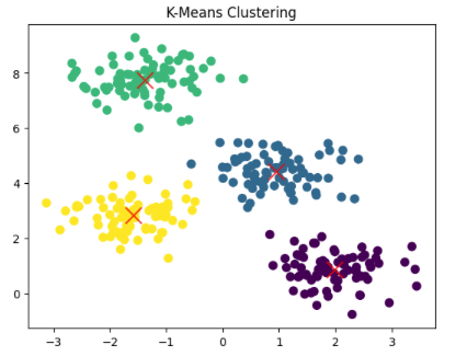
The final step is to visualize the clustered data points. Each cluster is represented using a different color, making it easier to observe how the algorithm separates the dataset into distinct groups.

The cluster centroids are highlighted using large red X markers. These centroids represent the central points around which similar observations are grouped.

# Plot clustered data points
plt.scatter(
    X[:, 0],
    X[:, 1],
    c=y_kmeans,
    s=50,
    cmap='viridis')

# Plot cluster centroids
centers = kmeans.cluster_centers_
plt.scatter(
    centers[:, 0],
    centers[:, 1],
    c='red',
    s=200,
    alpha=0.75,
    marker='X')

plt.title('K-Means Clustering')
plt.xlabel('Feature 1')
plt.ylabel('Feature 2')
plt.show()

Once the program is executed, the visualization displays multiple colored clusters formed automatically by the K-Means algorithm. Data points belonging to the same cluster appear with the same color, while the red X markers indicate the centroid positions.

2. Hierarchical Clustering

Machine Learning Hierarchical Clustering is a popular unsupervised machine learning technique used to group similar data points into clusters based on their similarity or distance from one another. Unlike K-Means Clustering, hierarchical clustering does not require specifying the number of clusters beforehand. Instead, it builds a hierarchy of clusters represented using a tree-like structure known as a dendrogram.

The algorithm works by progressively merging or splitting clusters based on similarity measures. Because of its ability to reveal relationships between data points at multiple levels, hierarchical clustering is widely used in bioinformatics, customer segmentation, document analysis, and pattern recognition tasks.

Hierarchical clustering can be performed using two approaches: agglomerative clustering and divisive clustering. Agglomerative clustering is the more commonly used method and follows a bottom-up approach. Initially, every data point is treated as its own cluster, after which the algorithm repeatedly merges the closest clusters until all points belong to a single cluster.

The clustering process relies heavily on distance metrics such as Euclidean distance and linkage methods that determine how distances between clusters are calculated.

The overall workflow of hierarchical clustering can be summarized as follows:

• Treat each data point as an individual cluster

• Compute distances between all clusters

• Merge the two closest clusters

• Repeat the merging process until a hierarchy is formed

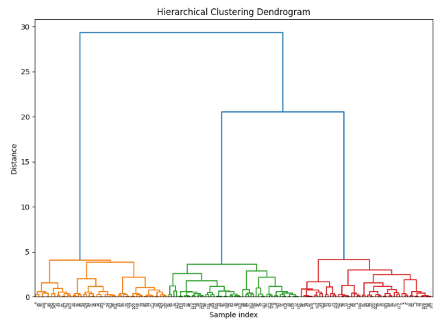
The resulting hierarchy is visualized using a dendrogram, where the height of each merge represents the distance between clusters. By cutting the dendrogram at a specific level, different cluster groupings can be obtained.

Implementation Hierarchical Clustering in Python

Now we will perform Hierarchical Clustering using the SciPy library and visualize the clustering hierarchy using a dendrogram. Unlike traditional clustering visualizations that only display grouped data points, a dendrogram provides a complete hierarchical representation of how clusters are formed during the clustering process.

The example below demonstrates how hierarchical clustering progressively merges similar observations together based on their distances. The implementation is divided into multiple stages to better understand each step involved in the clustering workflow.

Step 1: Importing the Required Libraries

The first step is to import all the required libraries. The linkage() function is used to perform hierarchical clustering, while the dendrogram() function helps visualize the hierarchical structure of the clusters. We also import Matplotlib for plotting the results.

from scipy.cluster.hierarchy import dendrogram, linkage
import matplotlib.pyplot as plt
from sklearn.datasets import make_blobs

Step 2: Generating Sample Data

Before applying the clustering algorithm, synthetic sample data is generated using the make_blobs() function. In this example, 150 data points are created around 3 different cluster centers.

The cluster_std parameter controls the spread of the clusters, while random_state ensures reproducibility of the generated dataset.

# Generate sample data
X, y = make_blobs(
    n_samples=150,
    centers=3,
    cluster_std=0.50,
    random_state=0)

Step 3: Performing Hierarchical Clustering

Next, hierarchical clustering is performed using the linkage() function. The 'ward' linkage method is used in this example, which minimizes the variance between clusters during the merging process.

The output stored in Z contains the hierarchical clustering information required to construct the dendrogram.

# Perform hierarchical clustering
Z = linkage(X, 'ward')

Step 4: Visualizing the Dendrogram

Finally, the dendrogram is plotted to visualize the hierarchical relationships between data points and clusters. The vertical lines in the dendrogram represent cluster merges, while the height of each merge indicates the distance between clusters.

# Plot dendrogram
plt.figure(figsize=(10, 7))
dendrogram(Z)
plt.title('Hierarchical Clustering Dendrogram')
plt.xlabel('Sample Index')
plt.ylabel('Distance')
plt.show()

The following dendrogram displays how clusters are progressively merged together during the hierarchical clustering process. Clusters that merge at lower heights are more similar to each other, while clusters connected at higher distances are less similar.

3. DBSCAN (Density-Based Spatial Clustering of Applications with Noise)

DBSCAN, short for Density-Based Spatial Clustering of Applications with Noise, is a powerful clustering algorithm designed to identify clusters based on the density of data points. Unlike algorithms such as K-Means, DBSCAN does not require the number of clusters to be specified beforehand. Instead, it automatically discovers clusters by analyzing how densely packed the data points are in different regions of the dataset.

One of the biggest advantages of DBSCAN is its ability to identify clusters with irregular shapes while also detecting outliers and noisy observations. Because of this, the algorithm is widely used in anomaly detection, geographic analysis, computer vision, and spatial data mining applications.

DBSCAN groups data points together by examining the density of neighboring observations around each point. The algorithm relies on two important parameters: eps and min_samples.

The eps parameter defines the radius within which neighboring points are searched, while min_samples specifies the minimum number of nearby points required for a region to be considered dense enough to form a cluster.

The overall clustering process can be summarized as follows:

• Identify neighboring points within a specified radius (eps)

• Classify points with sufficient neighbors as core points

• Expand clusters by connecting nearby dense regions

• Mark isolated points as noise or outliers

Points located in sparse regions that fail to satisfy the minimum density requirement are classified as noise. This makes DBSCAN particularly effective for datasets containing anomalies or irregular cluster structures.

Applications of DBSCAN Clustering

DBSCAN is widely used in scenarios where clusters may have arbitrary shapes or when noisy observations need to be detected automatically. In anomaly detection systems, the algorithm helps identify unusual transactions, fraudulent behavior, or abnormal sensor readings.

In geographic data analysis, DBSCAN is commonly used to identify densely populated regions, traffic hotspots, or spatial activity patterns. The algorithm is also useful in recommendation systems and market basket analysis for discovering groups of related behaviors.

Some major applications of DBSCAN include:

• Anomaly detection

• Geographic data analysis

• Market basket analysis

• Image segmentation

• Fraud detection

Because DBSCAN can effectively separate noise from meaningful clusters, it is highly valuable in real-world datasets where clean cluster boundaries rarely exist.

Implementation of DBSCAN Clustering in Python

We will use the scikit-learn library to apply DBSCAN Clustering on a synthetic dataset. The example demonstrates how density-based clustering can automatically identify groups of related data points while detecting outliers.

The implementation is divided into multiple stages for better understanding of the clustering workflow.

Step 1: Importing the Required Libraries

The first step is to import all the necessary libraries for clustering, numerical operations, data generation, and visualization.

from sklearn.cluster import DBSCAN
from sklearn.datasets import make_blobs
import matplotlib.pyplot as plt
import numpy as np

Step 2: Generating Sample Data

Before applying the DBSCAN algorithm, synthetic data points are generated using the make_blobs() function. The dataset contains 300 observations distributed around four cluster centers.

# Generate sample data
X, y = make_blobs(
    n_samples=300,
    centers=4,
    cluster_std=0.50,
    random_state=0)

Step 3: Applying the DBSCAN Algorithm

Next, the DBSCAN model is initialized using the eps and min_samples parameters. The fit_predict() method trains the model and simultaneously assigns cluster labels to the data points.

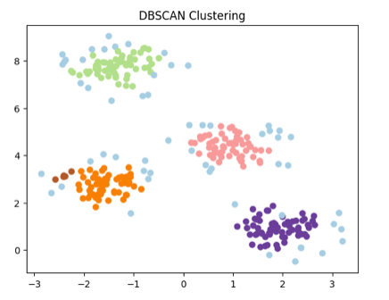
Points labeled as -1 are considered noise points or outliers by the algorithm.

# Apply DBSCAN
dbscan = DBSCAN(
    eps=0.3,
    min_samples=5)

# Predict cluster labels
y_dbscan = dbscan.fit_predict(X)

Step 4: Visualizing the Clusters

Finally, the clustered data points are visualized using a scatter plot. Different colors represent different clusters identified by the DBSCAN algorithm.

# Plot the clusters
plt.scatter(
    X[:, 0],
    X[:, 1],
    c=y_dbscan,
    cmap='Paired')

plt.title('DBSCAN Clustering')
plt.xlabel('Feature 1')
plt.ylabel('Feature 2')
plt.show()

Visualization from the output for the above code displays multiple clusters formed based on data density rather than centroid positions. Points belonging to the same dense region appear in the same color, while noisy observations may appear separately.

4. Mean Shift Algorithm

Mean Shift is a non-parametric clustering algorithm that identifies clusters by locating dense regions within the dataset. Unlike algorithms such as K-Means, Mean Shift does not require the number of clusters to be specified beforehand. Instead, it automatically discovers cluster centers by iteratively moving data points toward areas with higher data density.

The algorithm works by treating data points as samples from an underlying probability density function and gradually shifting candidate centroids toward the modes, or peaks, of that distribution. Because of this density-based approach, Mean Shift is highly effective for identifying arbitrarily shaped clusters and complex data structures.

Mean Shift begins by selecting initial candidate centroids from the dataset. For each centroid, the algorithm computes the mean position of all neighboring points located within a specified radius known as the bandwidth. The centroid is then shifted toward this newly computed mean position.

This process repeats iteratively until the centroid positions stabilize and convergence is achieved. Data points whose trajectories converge toward the same mode are grouped into the same cluster.

The overall workflow of Mean Shift Clustering can be summarized as follows:

• Initialize candidate centroids from the dataset

• Compute neighboring points within a defined bandwidth

• Shift centroids toward the mean position of nearby points

• Repeat the process until convergence is achieved

The bandwidth parameter plays a crucial role in determining the quality of clustering. Smaller bandwidth values may create many small clusters, while larger bandwidth values can merge clusters together.

Implementation Mean Shift in Python

In this implementation, we will use the scikit-learn library to perform Mean Shift Clustering on a synthetic dataset. The example demonstrates how the algorithm automatically identifies cluster centers by analyzing dense regions within the data.

The implementation is divided into multiple stages for better understanding of the clustering workflow.

Step 1: Importing the Required Libraries

The first step is to import all the necessary libraries required for clustering, visualization, and synthetic data generation.

from sklearn.cluster import MeanShift
from sklearn.datasets import make_blobs
import matplotlib.pyplot as plt

Step 2: Generating Sample Data

Next, synthetic sample data is generated using the make_blobs() function. The dataset contains 300 observations distributed across three cluster centers.

# Generate sample data
X, y = make_blobs(
    n_samples=300,
    centers=3,
    cluster_std=0.60,
    random_state=0)

Step 3: Applying the Mean Shift Algorithm

The Mean Shift model is initialized using the bandwidth parameter, which determines the search radius used for density estimation. The fit_predict() method trains the model and assigns cluster labels to each data point.

# Apply Mean Shift
meanshift = MeanShift(
    bandwidth=1)
# Predict cluster labels
y_meanshift = meanshift.fit_predict(X)

Step 4: Visualizing the Clusters

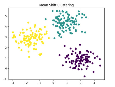
Finally, the clustered data points are visualized using a scatter plot. Different colors represent different clusters identified by the Mean Shift algorithm.

# Plot the cluster
splt.scatter(
    X[:, 0],
    X[:, 1],
    c=y_meanshift,
    cmap='viridis')

plt.title('Mean Shift Clustering')
plt.xlabel('Feature 1')
plt.ylabel('Feature 2')
plt.show()

The visualization displays clusters formed around dense regions of the dataset. Points belonging to the same density peak appear in the same color, illustrating how the algorithm groups observations based on local density distributions.

5. Gaussian Mixture Models (GMM)

Gaussian Mixture Models (GMM) are a probabilistic clustering technique used to model datasets as a combination of multiple Gaussian distributions. Unlike K-Means Clustering, which assigns each data point strictly to a single cluster, GMM provides soft clustering, meaning a data point can belong to multiple clusters with different probabilities.

This probabilistic approach allows Gaussian Mixture Models to capture more complex cluster structures, including overlapping and elliptical clusters. Because of this flexibility, GMM is widely used in pattern recognition, speech processing, image segmentation, and anomaly detection applications.

Gaussian Mixture Models assume that the dataset is generated from multiple Gaussian distributions, each representing a separate cluster. Every Gaussian distribution is defined by parameters such as mean, covariance, and mixture weight.

The algorithm typically uses the Expectation-Maximization (EM) algorithm to estimate these parameters iteratively. During the expectation step, probabilities are assigned to data points for belonging to different Gaussian distributions. In the maximization step, the model updates the distribution parameters to better fit the dataset.

The overall workflow of Gaussian Mixture Models can be summarized as follows:

• Assign probabilities of data points belonging to Gaussian distributions

• Estimate distribution parameters such as mean and covariance

• Update parameters using the Expectation-Maximization algorithm

• Repeat the process until convergence is achieved

Unlike centroid-based clustering algorithms, GMM can model clusters with varying shapes, sizes, and orientations, making it significantly more flexible for complex datasets.

Implementation of Gaussian Mixture Models in Python

In this implementation, we will use the scikit-learn library to apply Gaussian Mixture Model clustering on a synthetic dataset. The example demonstrates how probabilistic clustering can identify hidden structures within unlabeled data.

The implementation is divided into multiple stages for better understanding of the clustering process.

Step 1: Importing the Required Libraries

The first step is to import the required libraries for clustering, visualization, and synthetic data generation.

from sklearn.mixture import GaussianMixture
from sklearn.datasets import make_blobs
import matplotlib.pyplot as plt

Step 2: Generating Sample Data

Next, synthetic sample data is generated using the make_blobs() function. The dataset contains 300 observations distributed around three cluster centers.

# Generate sample data
X, y = make_blobs(
    n_samples=300,
    centers=3,
    cluster_std=0.60,
    random_state=0)

Step 3: Applying the Gaussian Mixture Model

The Gaussian Mixture Model is initialized using the n_components parameter, which specifies the number of Gaussian distributions to be used. The model is then trained using the fit() method, while the predict() method assigns cluster labels to each observation.

# Apply Gaussian Mixture Model
gmm = GaussianMixture(
    n_components=3,
    random_state=0)

# Train the model
gmm.fit(X)

# Predict cluster labels
y_gmm = gmm.predict(X)

Step 4: Visualizing the Clusters

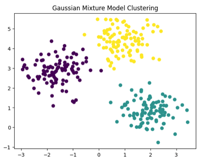
Finally, the clustered data points are visualized using a scatter plot. Different colors represent different clusters identified by the Gaussian Mixture Model.

# Plot the clusters
plt.scatter(
    X[:, 0],
    X[:, 1],
    c=y_gmm,
    cmap='viridis')

plt.title('Gaussian Mixture Model Clustering')
plt.xlabel('Feature 1')
plt.ylabel('Feature 2')
plt.show()

After executing the program, the visualization displays clusters formed by the Gaussian Mixture Model based on probabilistic distributions rather than strict centroid boundaries. Data points are grouped according to the Gaussian distribution they most likely belong to.

Conclusion

Clustering algorithms are essential tools in machine learning and data analysis, offering valuable insights by grouping data based on similarity. Each algorithm has its strengths and ideal use cases, depending on the nature of the data and the desired outcome. Python, with its rich ecosystem of libraries like scikit-learn, makes it easy to implement and experiment with these algorithms. Whether you're working on customer segmentation, anomaly detection, or image analysis, mastering these clustering techniques will undoubtedly enhance your data science skill set and open up new possibilities for data exploration and pattern discovery.