Machine Learning: What is Supervised Learning?

Supervised learning is a core technique in machine learning where models are trained on labeled data .i.e. data that includes both input features and the correct output. By learning the relationship between inputs and outputs, the algorithm can make accurate predictions on new, unseen data. It's widely used in applications like email spam detection, image classification, and stock price prediction.

In this blog, we’ll explore how supervised learning works, understand the core idea behind training models using labeled data, and examine some of the most widely used supervised learning algorithms including Logistic Regression, Decision Tree Learning, K-Nearest Neighbors Algorithm, and Support Vector Machine. Along the way, we’ll also build practical implementations in Python, visualize decision boundaries, and compare how different models learn patterns from data.

What is Supervised Machine learning?

Humans aren't born with many skills and we need to learn how to sort mail, land airplanes and have friendly conversations. Computer scientists have tried to help computers learn like we do with a process called supervised learning. The process of learning is how anything can make decisions. For example humans, animals or AI systems they can adapt their behavior based on their experiences. There are three main types of learning reinforcement, unsupervised and supervised learning. Supervised learning is the process of learning with training labels. It's the most widely used kind of learning when it comes to AI and it's what we will focus on in this blog.

Supervised learning is when someone who knows the right answer calls a supervisor, points out mistakes during the learning process. You can think of this like when a teacher corrects a student's math is one kind of supervised setting. We want AI to consider data like an image of an animal and classify it with a label like reptile or mammal. AI needs computing power and data to learn and that's especially true for supervised learning which needs a lot of training examples from a supervisor. After training this hypothetical AI it should be able to correctly classify images it hasn't seen before like a picture of a kitten as a mammal. That's how we know it's learning instead of just memorizing answers and supervised learning is a key part of lots of AI we interact with every day. 

• It's how email accounts can correctly classify a message from your boss as important and adds as spam. 

• It's how facebook tells your face apart from your friend's face so that it can make tax suggestions when you upload a photo 

• It's how your bank may decide whether your loan request is approved or not. 

Now to initially create this kind of AI computer scientists were loosely inspired by human brains they were mostly interested in cells called neurons because our brains have billions of them each neuron has three basic parts 

1. Cell body 

2. Dendrites 

3. Axon

The axon of one neuron is separated from the dendrites of another neuron by a small gap called a synapse and neurons talk to each other by passing electric signals through synapses as one neuron receives signals from another neuron. The electric energy inside of its cell body builds up until a threshold is crossed, then an electric signal shoots down the axon and is passed to another neuron where everything repeats. The goal of early computer scientists wasn't to mimic a whole brain, their goal was to create one artificial neuron that worked like a real one. 

How did ML come about?

In 1958 a psychologist named Frank Rosenblatt was determined to create an artificial neuron. His goal was to teach this AI to classify images as triangles or not triangles with his supervision. That's what makes it supervised learning.

The machine he built was about the size of a grand piano and he called it the perceptron. Rosenblatt wired the perceptron to a four hundred pixel camera which was quite high tech for the time, but is about a billion times less powerful than the one on the back of your modern cellphone. He would show the camera a picture of a triangle or a not triangle like a circle depending on if the camera saw ink or paper in each spot, each pixel would send a different electric signal to the perceptron then the perceptron would add up all the signals that match the triangle shape. If the total charge was above its threshold it would send an electric signal to turn on a light that was an artificial neuron speaking for yes that's a triangle.

But if the electric charge was too weak to hit the threshold it wouldn't do anything and the light wouldn't turn on that meant not a triangle. At first the perceptron was basically making random guesses so to turn it with supervision rosenblatt used yes and no buttons if the perceptron was correct, he would push the yes button and nothing would change but if the perceptron was wrong he would push the no button which set off a chain of events that adjusted how much electricity across the synapses and adjusted the machine's threshold levels so it'd be more likely to get the answer correct next time.

Nowadays, rather than building huge machines with switches and lights, we can use modern computers to program AI to behave like neurons. The basic concepts are pretty much the same. First the artificial neuron receives inputs multiplied by different weights which correspond to the strength of each signal in our brains. The electric signals between neurons are all the same size but with computers they can vary. The threshold is represented by a special weight called the bias which can be adjusted to raise or lower the neuron's eagerness to fire so all the inputs are multiplied by their respective weights added together and a mathematical function gets a result.

In the simplest AI systems this function is called a step function, which can only output a zero or a one if the sum is less than the bias then the neuron will output a zero which could indicate no triangle or something different depending on the task. But if the sum is greater than the bias then the neuron will output a one which indicates the opposite result. AI can be trained to make simple decisions about anything where you have enough data and supervised labels like triangles, junk mail languages, movie genres or even similar looking foods like doughnuts and bagels. 

List of Supervised Learning Algorithms

Supervised machine learning algorithms learn the patterns and different relationships between feature set and output data. These kind of algorithms are defined by there use of labeled data. A labeled data is a dataset that contains a lot of examples of Features and Target. Supervised learning uses algorithms that learn the relationship of Features and Target from the dataset. This process is referred to as Training or Fitting. A bunch of such supervised learning algorithms are given below:

1. Linear Regression

2. Logistic Regression

3. Decision Tree

4. SVM (Support Vector Machine)

5. Naive Bayes

6. kNN (k- Nearest Neighbors)

7. K-Means

8. Random Forest

9. Dimensionality Reduction Algorithms

10. Gradient Boosting Algorithms

Python Implementation of few Supervised learning Algorithms

Supervised learning is all about teaching machines using labeled data. In this hands-on tutorial, we’ll implement four essential supervised learning algorithms using Python and scikit-learn:

• Logistic Regression

• Decision Tree Classifier

• K-Nearest Neighbors (KNN)

• Support Vector Machine (SVM)

We’ll use a synthetic dataset so that we can easily visualize and understand how each algorithm separates data points. Let’s begin!

Step 1: Setup and Import Libraries

First, let’s import the necessary libraries. We’ll use scikit-learn for building supervised learning models, pandas and numpy for handling and processing data, and matplotlib along with seaborn for creating visualizations. These libraries form the backbone of many machine learning workflows in Python and help simplify everything from data preprocessing to model evaluation.

# Run this cell first
import numpy as np
import pandas as pd
import matplotlib.pyplot as plt
import seaborn as sns

from sklearn.datasets import make_classification
from sklearn.model_selection import train_test_split
from sklearn.preprocessing import StandardScaler
from sklearn.metrics import classification_report

from sklearn.linear_model import LogisticRegression
from sklearn.tree import DecisionTreeClassifier
from sklearn.neighbors import KNeighborsClassifier
from sklearn.svm import SVC

sns.set(style="whitegrid")

Step 2: Generate a Synthetic Classification Dataset

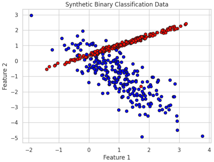
To understand these algorithms visually, we’ll generate a simple 2D classification dataset using make_classification. This will help us see the decision boundaries clearly when we plot them later.

# Create a binary classification dataset
X, y = make_classification(n_samples=500, n_features=2, n_informative=2,n_redundant=0, n_clusters_per_class=1,
random_state=42)

# Visualize the dataset
plt.figure(figsize=(7,5))
plt.scatter(X[:,0], X[:,1], c=y, cmap='bwr', edgecolor='k')
plt.title("Synthetic Binary Classification Data")
plt.xlabel("Feature 1")
plt.ylabel("Feature 2")
plt.show()

Output:

Step 3: Preprocess the Data

Before feeding the data into our models, we split it into training and testing sets. We also apply feature scaling to ensure that models like KNN and SVM perform optimally.

# Split into train and test
X_train, X_test, y_train, y_test = train_test_split(X, y, test_size=0.3, random_state=42)

# Feature scaling
scaler = StandardScaler()
X_train_scaled = scaler.fit_transform(X_train)
X_test_scaled = scaler.transform(X_test)

1. Logistic Regression

Logistic Regression is one of the most widely used supervised learning algorithms for binary classification problems. Despite the name, it is actually used for classification rather than regression. The model learns a linear decision boundary that separates data points into different classes based on probability.

Internally, logistic regression applies a sigmoid function to transform predictions into probability scores between 0 and 1. If the predicted probability crosses a certain threshold, the sample is assigned to a particular class. Simple, efficient, interpretable.

log_model = LogisticRegression()
log_model.fit(X_train_scaled, y_train)

y_pred_log = log_model.predict(X_test_scaled)

print("🔍 Logistic Regression Report:\n")
print(classification_report(y_test, y_pred_log))

The classification report provides several important evaluation metrics that help measure the performance of the model. Precision indicates how many predicted positive samples were actually correct, while recall measures how many actual positive samples were successfully identified by the model.

The F1-score combines both precision and recall into a single metric by calculating their harmonic mean, making it especially useful when dealing with imbalanced datasets. Accuracy represents the overall percentage of correctly classified predictions across the dataset.

2. Decision Tree Classifier

Decision Tree Learning is a supervised learning algorithm that classifies data by recursively splitting the dataset into smaller regions based on feature conditions. Each internal node in the tree represents a decision rule, while the leaf nodes represent the final predicted classes. Unlike linear models, decision trees can capture complex and non-linear relationships within the data, making them highly flexible and easy to interpret.

The model works by selecting feature thresholds that best separate the classes at each step, gradually building a tree-like structure of decisions. One branch at a time, the algorithm keeps dividing the dataset until it reaches a stopping condition.

tree_model = DecisionTreeClassifier(max_depth=4)
tree_model.fit(X_train, y_train)

y_pred_tree = tree_model.predict(X_test)

print("🌳 Decision Tree Report:\n")
print(classification_report(y_test, y_pred_tree))

Output:

3. K-Nearest Neighbors (KNN)

K-Nearest Neighbors Algorithm is a supervised learning algorithm that classifies data points based on the labels of their nearest neighboring samples. Instead of learning an explicit mathematical model during training, KNN stores the training data and makes predictions by measuring distances between data points. It is considered a non-parametric and instance-based learning method because it relies directly on the dataset during inference.

When a new sample is introduced, the algorithm identifies the k closest neighbors and assigns the class that appears most frequently among them. In this implementation, we use k = 5, meaning the prediction is based on the majority vote of the five nearest data points. Tiny local democracy operating entirely on Euclidean distance. Civilization distilled into geometry.

Since KNN depends heavily on distance calculations, feature scaling becomes extremely important. Without normalization, features with larger numerical ranges can dominate the distance metric and negatively affect predictions.

knn_model = KNeighborsClassifier(n_neighbors=5)
knn_model.fit(X_train_scaled, y_train)

y_pred_knn = knn_model.predict(X_test_scaled)

print("📍 KNN Report:\n")
print(classification_report(y_test, y_pred_knn))

Output:

4. Support Vector Machine (SVM)

Support Vector Machine is a powerful supervised learning algorithm used for both classification and regression tasks. The main objective of SVM is to find the optimal hyperplane that separates different classes while maximizing the margin between them. A larger margin generally improves the model’s ability to generalize to unseen data.

Support vectors are the critical data points located closest to the decision boundary, and they directly influence the position of the separating hyperplane.

SVM can handle both linear and non-linear classification problems through the use of different kernel functions such as linear, polynomial, and radial basis function (RBF) kernels.

svm_model = SVC(kernel='linear')
svm_model.fit(X_train_scaled, y_train)

y_pred_svm = svm_model.predict(X_test_scaled)

print("💻 SVM Report:\n")
print(classification_report(y_test, y_pred_svm))

Output:

Step 4: Visualize Decision Boundaries

Some models create simple linear boundaries, while others produce highly flexible and non-linear regions depending on the complexity of the algorithm and the structure of the dataset. Visualizing these boundaries makes it easier to compare how different models learn patterns from the same data. It also reveals issues such as overfitting, underfitting, and poor class separation. In other words, colorful geometric evidence of a model either understanding the data or hallucinating confidence with remarkable enthusiasm.

To simplify the visualization process, we’ll define a reusable function that generates decision boundary plots for different classifiers.

def plot_decision_boundary(model, X, y, title, scale=True):
    x_min, x_max = X[:, 0].min() - .5, X[:, 0].max() + .5
    y_min, y_max = X[:, 1].min() - .5, X[:, 1].max() + .5
    h = 0.01
    xx, yy = np.meshgrid(np.arange(x_min, x_max, h),
                         np.arange(y_min, y_max, h))
    X_grid = np.c_[xx.ravel(), yy.ravel()]
    if scale:
        X_grid = scaler.transform(X_grid)
    
    Z = model.predict(X_grid)
    Z = Z.reshape(xx.shape)
    
    plt.figure(figsize=(7,5))
    plt.contourf(xx, yy, Z, alpha=0.4, cmap='bwr')
    plt.scatter(X[:, 0], X[:, 1], c=y, edgecolors='k', cmap='bwr')
    plt.title(title)
    plt.xlabel("Feature 1")
    plt.ylabel("Feature 2")
    plt.show()

Step 5: Plotting Decision Boundaries for Each Model

Now that the visualization function is ready, we can plot the decision boundaries for each supervised learning algorithm and compare how they classify the dataset in two-dimensional feature space. These plots provide an intuitive understanding of how different models learn patterns and separate classes.

Linear models such as Logistic Regression and linear SVM typically create straight decision boundaries, while algorithms like Decision Trees and K-Nearest Neighbors can generate more flexible and non-linear regions depending on the structure of the data.

plot_decision_boundary(log_model, X, y, "Logistic Regression", scale=True)
plot_decision_boundary(tree_model, X, y, "Decision Tree", scale=False)
plot_decision_boundary(knn_model, X, y, "K-Nearest Neighbors", scale=True)
plot_decision_boundary(svm_model, X, y, "Support Vector Machine", scale=True)

The Logistic Regression model creates a linear decision boundary that separates the two classes using a straight line. Since it assumes a linear relationship between the features and the target variable, the separation region appears smooth and simple. The model performs well when the classes are approximately linearly separable.

The Decision Tree classifier divides the feature space into rectangular regions using a series of hierarchical decision rules. Unlike linear models, it can capture non-linear relationships by creating multiple splits based on feature thresholds. This results in block-like decision boundaries that adapt more flexibly to the dataset.

The KNN classifier generates highly flexible and non-linear decision boundaries based on the local distribution of neighboring data points. Instead of learning a global decision function, it classifies each sample using nearby observations, which allows it to adapt closely to the shape of the data. The irregular boundary reflects its sensitivity to local patterns in the dataset.

The Support Vector Machine creates a clear linear decision boundary that separates the two classes while maximizing the margin between them. The red and blue shaded regions represent the predicted classification areas for each class, while the straight boundary line reflects the optimal hyperplane learned by the model.

Conclusion

Supervised learning remains one of the most important pillars of machine learning and artificial intelligence because of its ability to learn meaningful patterns from labeled data and make accurate predictions on unseen information. From simple linear classifiers to more advanced non-linear models, supervised algorithms power a wide range of real-world applications including fraud detection, recommendation systems, medical diagnosis, image recognition, and intelligent automation.

As datasets continue to grow in scale and complexity, supervised learning techniques continue evolving alongside modern AI systems, forming the foundation for many advanced deep learning and predictive analytics applications. Understanding how these models learn, generalize, and make decisions is essential for building reliable and efficient machine learning solutions in both research and industry. Beneath the layers of mathematical optimization and polished AI terminology, supervised learning is ultimately about teaching systems to recognize patterns well enough to make informed decisions.